物理与统计:从零开始Physics and statistics from zero
这一页把项目需要的全部物理与统计从一年级水平讲起。每一节先给概念,再给一个算得出来的数字例子,再给一张图。读完你应该能自己解释:为什么一台光栅光谱仪会把空间信息混进波长里,为什么这对超新星遗迹是致命的,以及为什么最后必须用一个带讨厌参数的似然拟合才能把两者分开。This page builds up all the physics and statistics the project needs, starting from first-year level. Each section gives the concept, then a number example you can compute, then a figure. Afterwards you should be able to explain yourself why a grating spectrometer mixes spatial information into wavelength, why that is fatal for a supernova remnant, and why only a likelihood fit with nuisance parameters can separate the two.
本页目录On this page
- 一台光栅光谱仪:色散与交叉色散A grating spectrometer: dispersion and cross-dispersion
- 展源:为什么位置与波长混在一起Extended sources: why position and wavelength mix
- 响应矩阵(RMF)与线扩散函数(LSF)The response matrix (RMF) and the line-spread function (LSF)
- 超新星遗迹与它的等离子体Supernova remnants and their plasma
- 泊松似然与 C 统计量The Poisson likelihood and the C-statistic
- 前向建模一个展源Forward modelling an extended source
- 讨厌参数Nuisance parameters
- Fisher 误差与轮廓似然Fisher errors and the profile likelihood
1. 一台光栅光谱仪:色散与交叉色散1. A grating spectrometer: dispersion and cross-dispersion
1.1 概念The concept
XMM-Newton 上的 RGS(Reflection Grating Spectrometer,反射光栅光谱仪)是一台无色散坐标与有色散坐标互相垂直的仪器。想象一块规整的反射光栅:入射的 X 射线光子按波长偏折,偏折方向叫色散方向(dispersion direction),偏折大小随波长单调变化。垂直的方向叫交叉色散方向(cross-dispersion direction),它对应天空上的空间位置,光栅不在这里分光。The RGS (Reflection Grating Spectrometer) on XMM-Newton is an instrument with two perpendicular detector coordinates. Picture a regular reflection grating: incoming X-ray photons are deflected by an amount that grows with wavelength, along the dispersion direction. The perpendicular direction is the cross-dispersion direction; it maps the spatial position on the sky and the grating does not disperse light there.
所以 RGS 的探测器读出是一张二维图:横轴(色散)是波长,纵轴(交叉色散)是空间。抽谱就是把纵轴切成若干条带(strip,也叫 XDSP 行),每条带沿横轴积成一条一维光谱。So the RGS detector read-out is a two-dimensional image: the horizontal axis (dispersion) is wavelength and the vertical axis (cross-dispersion) is position on the sky. Extraction cuts the vertical axis into strips (also called XDSP rows) and integrates each strip along the horizontal axis into a one-dimensional spectrum.
1.2 算一个数:色散定律A worked number: the dispersion law
项目在参考观测的中央条带上实测出色散定律:交叉色散方向每偏移 1 角分(arcmin),谱线在色散方向移动 0.1233 Å(E010,I015)。反过来,一个宽 0.75′ 的条带对应多长的波长区间?The project measured the dispersion law on the central strip of the reference observation: each arcmin of cross-dispersion offset moves a line by 0.1233 Angstrom along the dispersion axis (E010, I015). Conversely, what wavelength interval does a strip 0.75 arcmin wide cover?
\[ \Delta\lambda = 0.1233\ \frac{\mathrm{Å}}{\prime} \times 0.75\,\prime = 0.0925\ \mathrm{Å} \]\[ \Delta\lambda = 0.1233\ \frac{\mathrm{Å}}{\prime} \times 0.75\,\prime = 0.0925\ \mathrm{Å} \]
也就是说,N132D 分析里一条 0.75′ 宽的条带,只覆盖 0.0925 Å 的波长。O VII 三重线的三条线(21.60、21.81、22.10 Å)相隔约 0.2 Å,比一条带还宽,所以三条线落在不同的色散通道上,可以分开测。That is, one 0.75 arcmin strip in the N132D analysis covers only 0.0925 Angstrom of wavelength. The three lines of the O VII triplet (21.60, 21.81, 22.10 Angstrom) are about 0.2 Angstrom apart, wider than one strip, so they land in different dispersion channels and can be measured separately.
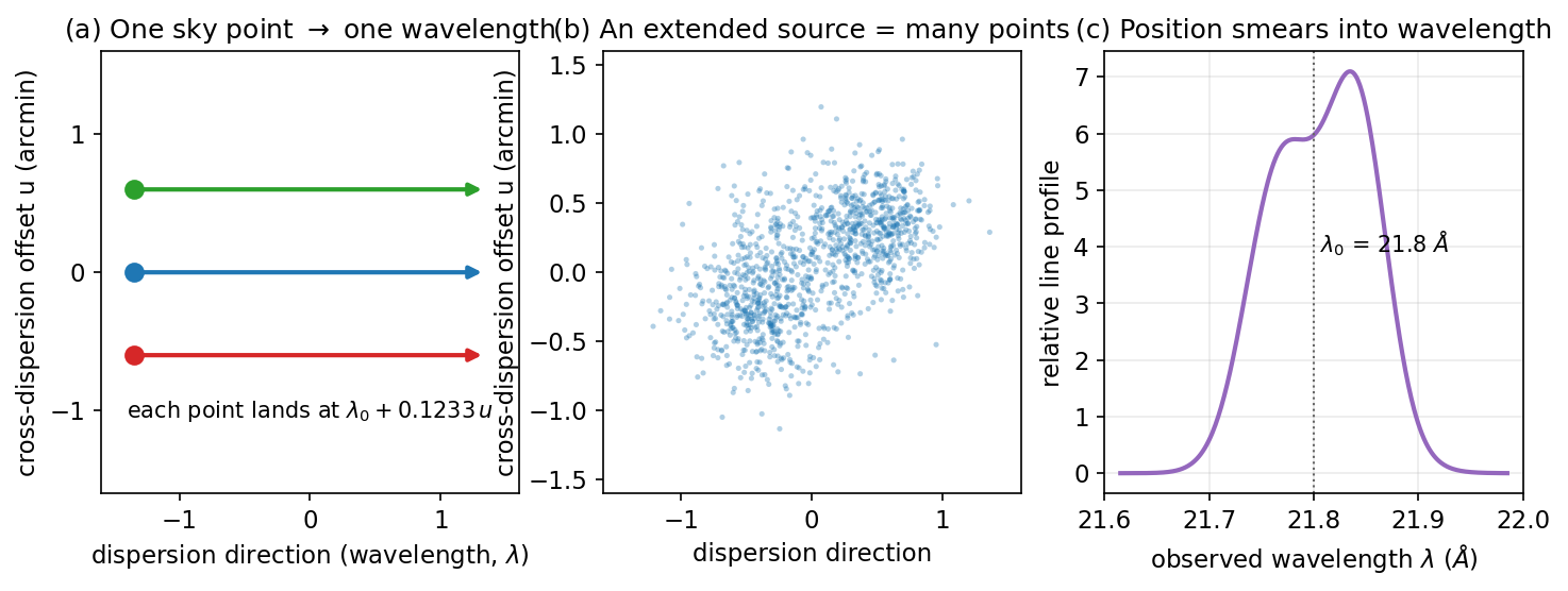
来源:色散定律 0.1233 Å/′ 来自 cognition-os/03_TRUST_TABLE.md E010 行(Trusted,范围:参考观测、中央条带);三个观测共同给出 0.1236–0.1238 Å/′(E014)。条带宽度 0.75′ 与三条线波长来自 .agent/jobs/2026-10-19-e018c-ovii-stage2/BRIEF.md 与 agent-memory/procedures.md(O VII He-alpha 三重线 21.60/21.81/22.10 Å,经 Suzuki et al. 2020 与 ATOMDB 3.0.9 核对)。Source: the dispersion law of 0.1233 Angstrom per arcmin is from cognition-os/03_TRUST_TABLE.md row E010 (Trusted, scope: the reference observation, central strip); the three observations together give 0.1236-0.1238 Angstrom per arcmin (E014). The strip width of 0.75 arcmin and the triplet wavelengths are from .agent/jobs/2026-10-19-e018c-ovii-stage2/BRIEF.md and agent-memory/procedures.md (O VII He-alpha triplet 21.60/21.81/22.10 Angstrom, checked against Suzuki et al. 2020 and ATOMDB 3.0.9).
2. 展源:为什么位置与波长混在一起2. Extended sources: why position and wavelength mix
2.1 概念The concept
对点源,交叉色散位置是已知常数,谱线位置只由波长决定,没有问题。对展源(N132D 在天上张好几角分),每个天空像素有自己的交叉色散位置,于是同一个波长的光子会落在不同的色散位置:天空位置被混进了波长轴。这就是项目要解决的核心困难。For a point source the cross-dispersion position is a known constant, so a line's position depends only on wavelength, and there is no problem. For an extended source (N132D spans several arcmin on the sky) every sky pixel has its own cross-dispersion position, so photons of the same wavelength land at different dispersion positions: sky position is mixed into the wavelength axis. This is the central difficulty the project solves.
更糟的是超新星遗迹本身在膨胀:不同位置的气体有不同视向速度,谱线本来就该随位置移动。所以“谱线随位置的移动”有两个来源——几何(色散定律)与物理(多普勒),单看一条光谱无法区分。It is worse still for a supernova remnant, which is itself expanding: gas at different positions has different line-of-sight velocities, so lines should move with position anyway. The "movement of a line with position" therefore has two origins, geometric (the dispersion law) and physical (Doppler), and a single spectrum cannot tell them apart.
2.2 算一个数:多普勒与几何谁大A worked number: Doppler versus geometry
非相对论多普勒:\(\Delta\lambda / \lambda = v / c\),其中 \(c = 299\,792.458\) km/s。取 O VII 线 \(\lambda = 21.8\) Å:Non-relativistic Doppler: \(\Delta\lambda / \lambda = v / c\), with \(c = 299\,792.458\) km/s. Take the O VII line at \(\lambda = 21.8\) Angstrom:
\[ v = 100\ \mathrm{km/s} \quad\Rightarrow\quad \Delta\lambda = \frac{100}{299\,792.458}\times 21.8\ \mathrm{Å} = 0.0073\ \mathrm{Å} \]\[ v = 100\ \mathrm{km/s} \quad\Rightarrow\quad \Delta\lambda = \frac{100}{299\,792.458}\times 21.8\ \mathrm{Å} = 0.0073\ \mathrm{Å} \]
而几何上,交叉色散移动 0.06′(约 3.6″,一个 XDSP 像素量级)带来的色散移动是:Geometrically, a cross-dispersion shift of 0.06 arcmin (about 3.6 arcsec, of order one XDSP pixel) moves the line by:
\[ \Delta\lambda_{\mathrm{geom}} = 0.1233\ \frac{\mathrm{Å}}{\prime}\times 0.06\,\prime = 0.0074\ \mathrm{Å} \]\[ \Delta\lambda_{\mathrm{geom}} = 0.1233\ \frac{\mathrm{Å}}{\prime}\times 0.06\,\prime = 0.0074\ \mathrm{Å} \]
来源:中央条带的接受度节点值取自 pack_0210681301.npz 的 probes[1, :, :, :](按入射行与通道求和);动画为线性插值示意。Source: the central strip's acceptance node values come from pack_0210681301.npz, probes[1, :, :, :] (summed over incident rows and channels); the animation is a linear-interpolation illustration.
两个数几乎相等。这正是 I021 报告的那个偏移(共同项 \(-6.25 \pm 0.49\)″)的物理意义:一个像素量级的空间错位,就能伪装成 100 km/s 的速度。所以必须把交叉色散偏移当讨厌参数拟掉,否则速度场不可信。The two numbers are almost equal. This is exactly the physical meaning of the offset reported in I021 (a common term of \(-6.25 \pm 0.49\) arcsec): a one-pixel spatial misplacement can masquerade as 100 km/s of velocity. The cross-dispersion offset must therefore be fitted out as a nuisance parameter, or the velocity field is not credible.
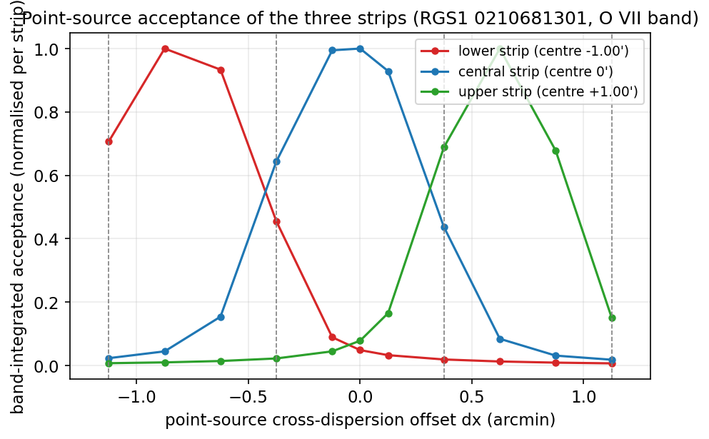
来源:/u/Lang3/Data/S2Fitting/verification/n132d-velfield-inputs-20261014/pack_0210681301.npz(probes[strip, dx, row, channel],条带中心 \(-0.75\)、\(0\)、\(+0.75\)′,节点在 \(1.125\)′)。多普勒换算与几何换算的数字由本页公式算出;I021 的偏移值见 cognition-os/03_TRUST_TABLE.md I021 行(Trusted,范围已收窄)。Source: /u/Lang3/Data/S2Fitting/verification/n132d-velfield-inputs-20261014/pack_0210681301.npz (probes[strip, dx, row, channel], strip centres -0.75, 0, +0.75 arcmin, nodes at 1.125 arcmin). The Doppler and geometric numbers follow from the formulas on this page; the I021 offset is from cognition-os/03_TRUST_TABLE.md row I021 (Trusted, narrowed scope).
来源:色散定律 0.1233 Å/′(E010,Trusted);示意图为本页 JS 动画,非科学证据。Source: the dispersion law of 0.1233 Angstrom per arcmin (E010, Trusted); the drawing is this page's JS animation, not scientific evidence.
3. 响应矩阵(RMF)与线扩散函数(LSF)3. The response matrix (RMF) and the line-spread function (LSF)
3.1 概念The concept
光谱仪不是把每个入射波长原样送到一个通道:它把能量为 \(E\) 的光子按概率分布撒到一串探测器通道上。这个“入射能量到通道”的概率表就是响应矩阵(RMF,redistribution matrix file)。把它与有效面积(ARF)相乘,就得到“每单位光子流在通道 \(k\) 产生的期望计数”。SAS 的 rgsrmfgen 为每个(源位置、条带)组合生成一个 RMF,所以展源需要 27 个(9 源格、3 条带)。A spectrometer does not deliver each incoming wavelength to one channel: it scatters a photon of energy \(E\) across a run of detector channels with fixed probabilities. That table of "incident energy to channel" is the response matrix (RMF, redistribution matrix file). Multiplied by the effective area (ARF) it gives "expected counts in channel \(k\) per unit photon flux". SAS's rgsrmfgen produces one RMF per (source position, strip) pair, so an extended source needs 27 of them (9 source cells, 3 strips).
单看一条谱线,RMF 沿通道的分布就是线扩散函数(LSF,line-spread function):一条无限窄的线会被仪器展宽。RGS 的 LSF 核心宽度在 O VII r 线处约 \(\sigma = 437\) km/s(I020)。这个宽度是仪器的,不是气体的:如果气体本身有速度弥散 \(\sigma_v\),观测到的线宽是两者的卷积(按方差相加)。Looking at one line, the RMF's distribution across channels is the line-spread function (LSF): an infinitely narrow line is broadened by the instrument. The RGS LSF core width at the O VII r line is about \(\sigma = 437\) km/s (I020). That width belongs to the instrument, not the gas: if the gas itself has a velocity dispersion \(\sigma_v\), the observed width is their convolution (variances add).
3.2 算一个数:837 km/s 的线宽里有多少是气体A worked number: how much of an 837 km/s line width is gas
如果测到的总宽是 \(\sigma_{\text{obs}} = 500\) km/s,而仪器贡献 \(\sigma_{\text{LSF}} = 437\) km/s,那么气体本身只有:If the total measured width is \(\sigma_{\text{obs}} = 500\) km/s and the instrument contributes \(\sigma_{\text{LSF}} = 437\) km/s, the gas alone has only:
\[ \sigma_v = \sqrt{\sigma_{\text{obs}}^2 - \sigma_{\text{LSF}}^2} = \sqrt{500^2 - 437^2} = 242\ \mathrm{km/s} \]\[ \sigma_v = \sqrt{\sigma_{\text{obs}}^2 - \sigma_{\text{LSF}}^2} = \sqrt{500^2 - 437^2} = 242\ \mathrm{km/s} \]
注意这个例子说明了为什么 LSF 标定是命门:仪器宽度差 2 %,\(\sigma_v\) 就偏 24 km/s(0.4 SD,I020)。项目的拟合不用减法去卷积,而是前向把高斯速度分布与 LSF 卷起来再与数据比,这样误差传播是干净的。Note this example shows why the LSF calibration is the crux: a 2 % error in the instrument width biases \(\sigma_v\) by 24 km/s (0.4 SD, I020). The project's fit does not deconvolve by subtraction; it forward-convolves the Gaussian velocity distribution with the LSF and compares with the data, so the error propagation is clean.
来源:cognition-os/03_TRUST_TABLE.md I020 行(Trusted;E018d Asimov mock,LSF 核心 \(\sigma\) 437 km/s;2 % 宽度误差使 \(\sigma_v\) 偏 \(+24\) km/s 即 0.4 SD;LSF 宽度无法由数据自行标定,corr \(-0.999\))。Source: cognition-os/03_TRUST_TABLE.md row I020 (Trusted; E018d Asimov mock, LSF core \(\sigma\) 437 km/s; a 2 % width error biases \(\sigma_v\) by \(+24\) km/s, 0.4 SD; the LSF width is not self-calibratable from the data, corr \(-0.999\)).
4. 超新星遗迹与它的等离子体4. Supernova remnants and their plasma
4.1 概念The concept
N132D 是大麦哲伦云(LMC)里一个约 2500 年的年轻超新星遗迹。恒星爆炸的激波把星际物质加热到百万度量级,形成碰撞电离的等离子体(collisional-ionisation equilibrium 还没达到,所以是 NEI,non-equilibrium ionisation)。这样的等离子体在软 X 射线(0.3–1 keV)发出很多谱线,其中最强的一族是氧:O VII(七次电离的氧,只剩一个电子,类氢氦结构)的 He-alpha 三重线(r、i、f 三条),和 O VIII(类氢,只剩一个电子)的 Ly-alpha 线。N132D is a young supernova remnant, about 2500 years old, in the Large Magellanic Cloud (LMC). The explosion's shock heats the interstellar medium to millions of degrees, forming a collisionally ionised plasma that has not yet reached equilibrium (so it is NEI, non-equilibrium ionisation). Such a plasma emits many lines in the soft X-ray band (0.3-1 keV); the strongest family is oxygen: the O VII He-alpha triplet (lines r, i and f) and the O VIII Ly-alpha line.
三重线的三条线有物理含义:r(resonance,共振线)来自允许跃迁,i(intercombination,交叉组合)与 f(forbidden,禁线)来自亚稳态。它们的强度比(G 比 \(= (f+i)/r\))对温度敏感,密度比(\(R = f/i\))对密度敏感。但本项目当前只把三条线当独立的自由振幅拟合——因为速度场是目标,不是等离子体诊断。The three lines carry physics: r (resonance) comes from an allowed transition, i (intercombination) and f (forbidden) from metastable levels. Their ratios (the G ratio \(= (f+i)/r\)) are temperature-sensitive, and the density ratio (\(R = f/i\)) is density-sensitive. This project, however, fits the three lines as three independent free amplitudes, because the target is the velocity field, not plasma diagnostics.
气体在膨胀,所以不同壳层位置的气体有不同的视向速度:正对我们的部分蓝移,背离的部分红移。把所有壳层的光加在一起,谱线就变宽——这就是 \(\sigma_v\) 的来源。如果壳层大体是一个膨胀球壳,那么“接近”与“远离”两个成分各占一半,中间重叠最多,观测到的线顶就会变平甚至双峰。这正是 E018b 第一阶段在亮条带里看到的形状(I029)。The gas is expanding, so gas at different shell positions has different line-of-sight velocities: the side facing us is blue-shifted and the far side red-shifted. Adding all the shell light together broadens the line, which is where \(\sigma_v\) comes from. If the shell is roughly an expanding sphere, the approaching and receding components each carry half the light and overlap most in the middle, so the observed line top flattens or even splits in two. That is exactly the shape seen in the bright strips in stage 1 of E018b (I029).
来源:谱线名与波长来自 agent-memory/procedures.md(经 Suzuki et al. 2020 与 ATOMDB 3.0.9 核对);线形读法来自 cognition-os/insights/I029_n132d-ovii-velocity-stage1.md(模型不足一节:亮条带谱线顶部平坦或双峰)。N132D 的年龄与 NEI 状态见 agent-memory/environment.md N132D 参考模型一节(Suzuki et al. 2020,bvrnei 三成分)。Source: line names and wavelengths from agent-memory/procedures.md (checked against Suzuki et al. 2020 and ATOMDB 3.0.9); the line-shape reading from cognition-os/insights/I029_n132d-ovii-velocity-stage1.md (model inadequacy: bright-strip line tops flat or double-peaked). N132D's age and NEI state are in agent-memory/environment.md, the N132D reference model section (Suzuki et al. 2020, three bvrnei components).
5. 泊松似然与 C 统计量5. The Poisson likelihood and the C-statistic
5.1 概念The concept
X 射线光子是逐个到达的:通道 \(k\) 里的计数 \(N_k\) 服从泊松分布,期望值 \(\mu_k(\theta)\) 由模型给出:X-ray photons arrive one at a time: the count \(N_k\) in channel \(k\) follows a Poisson distribution whose mean \(\mu_k(\theta)\) comes from the model:
\[ P(N_k \mid \mu_k) = \frac{\mu_k^{N_k} e^{-\mu_k}}{N_k !} \]\[ P(N_k \mid \mu_k) = \frac{\mu_k^{N_k} e^{-\mu_k}}{N_k !} \]
把所有通道(和所有观测、所有条带)的乘积取对数,就得到对数似然。习惯上用C 统计量(C-statistic,Cash 统计量):Taking the log of the product over all channels (and all observations and strips) gives the log-likelihood. By convention one uses the C-statistic (the Cash statistic):
\[ C = 2\sum_k \left[\,\mu_k(\theta) - N_k + N_k\ln\frac{N_k}{\mu_k(\theta)}\,\right] \]\[ C = 2\sum_k \left[\,\mu_k(\theta) - N_k + N_k\ln\frac{N_k}{\mu_k(\theta)}\,\right] \]
拟合就是找让 \(C\) 最小的参数 \(\theta\)。\(C\) 越小越好;两个嵌套模型差 \(\Delta C\) 服从 \(\chi^2\) 分布,自由度等于参数个数差。注意 \(N_k = 0\) 的通道也贡献 \(\mu_k\)(模型预测了光子但没看到),这是 C 统计量与 \(\chi^2\) 的关键区别之一。Fitting means finding the parameters \(\theta\) that minimise \(C\). Smaller \(C\) is better; the difference \(\Delta C\) between two nested models follows a \(\chi^2\) distribution with degrees of freedom equal to the difference in parameter count. Note that channels with \(N_k = 0\) still contribute \(\mu_k\) (the model predicts photons that were not seen), one of the key differences between the C-statistic and \(\chi^2\).
5.2 算一个数:一条谱线要多少光子A worked number: how many photons a line needs
泊松计数的相对误差是 \(1/\sqrt{N}\)。O1 观测中央条带 O VII 波段的总计数是 1325(E015 冻结包),所以:The relative error of a Poisson count is \(1/\sqrt{N}\). The O VII-band total count of the O1 central strip is 1325 (the frozen E015 pack), so:
\[ \frac{1}{\sqrt{1325}} = 2.75\,\% \]\[ \frac{1}{\sqrt{1325}} = 2.75\,\% \]
而三个观测合起来(2337 + 10274 + 20258 计数,E015 简报):And for the three observations together (2337 + 10274 + 20258 counts, the E015 brief):
\[ N_{\text{total}} = 32\,869, \qquad \frac{1}{\sqrt{N_{\text{total}}}} = 0.55\,\% \]\[ N_{\text{total}} = 32\,869, \qquad \frac{1}{\sqrt{N_{\text{total}}}} = 0.55\,\% \]
所以三个观测合起来统计上很强;限制来自系统误差(模板、LSF、响应),这也是为什么项目花大量力气在标定源上。So the three observations together are statistically strong; the limit comes from systematics (template, LSF, response), which is why the project invests so heavily in calibrators.
来源:计数来自 /u/Lang3/Data/S2Fitting/verification/n132d-velfield-inputs-20261014/ 的三个 pack_*.npz(本页图 2 同源;O1 中央条带 source_counts 总和 1325;三观测总和 2337/10274/20258 见 cognition-os/00_AI_BRIEFING.md E015 一节)。Source: the counts are from the three pack_*.npz files under /u/Lang3/Data/S2Fitting/verification/n132d-velfield-inputs-20261014/ (the same source as Figure 2; the O1 central strip's source_counts sum is 1325; the three-observation totals 2337/10274/20258 are in cognition-os/00_AI_BRIEFING.md, the E015 section).
6. 前向建模一个展源6. Forward modelling an extended source
6.1 概念The concept
既然观测到的光谱是“天空亮度乘仪器响应”的混合,最干净的做法是前向建模:先在天空上写下一个模型(模板图像、速度场),把它投影到每个观测的色散几何上,用响应矩阵折叠成每个条带的期望计数 \(\mu_k\),再与真实数据比。项目当前的天空模板是 Chandra 的 O VII 波段图像(0.50–0.62 keV),速度模型是“平面速度场 \(v = v_0 + \mathbf{g}\cdot\mathbf{x}\) 加一个高斯弥散 \(\sigma_v\)”。Since the observed spectrum is a mix of "sky brightness times instrument response", the cleanest approach is forward modelling: write down a model on the sky (a template image, a velocity field), project it onto each observation's dispersion geometry, fold it through the response matrices into expected counts \(\mu_k\) per strip, and compare with the real data. The project's current sky template is the Chandra O VII band image (0.50-0.62 keV), and the velocity model is "a plane velocity field \(v = v_0 + \mathbf{g}\cdot\mathbf{x}\) plus one Gaussian dispersion \(\sigma_v\)".
为什么用 Chandra 图像当模板?因为 RGS 自己没有空间分辨率去独立测量 N132D 的形态,而 Chandra 的 PSF 小得多。但 O VII 波段并不纯:Chandra 的 0.50–0.62 keV 图像里混着别的光子(O VII r 占 0.744,O VIII Ly-alpha 占 0.118,N VII Ly-alpha 占 0.647,I023),所以模板本身带一个约 0.22 SD 的污染系统误差(RT06 修订)。Why use a Chandra image as the template? Because the RGS itself has no spatial resolution to measure N132D's morphology independently, while Chandra's PSF is much smaller. But the O VII band is not pure: the Chandra 0.50-0.62 keV image contains other photons (0.744 of O VII r, 0.118 of O VIII Ly-alpha and 0.647 of N VII Ly-alpha, I023), so the template carries a contamination systematic of about 0.22 SD (the RT06 revision).
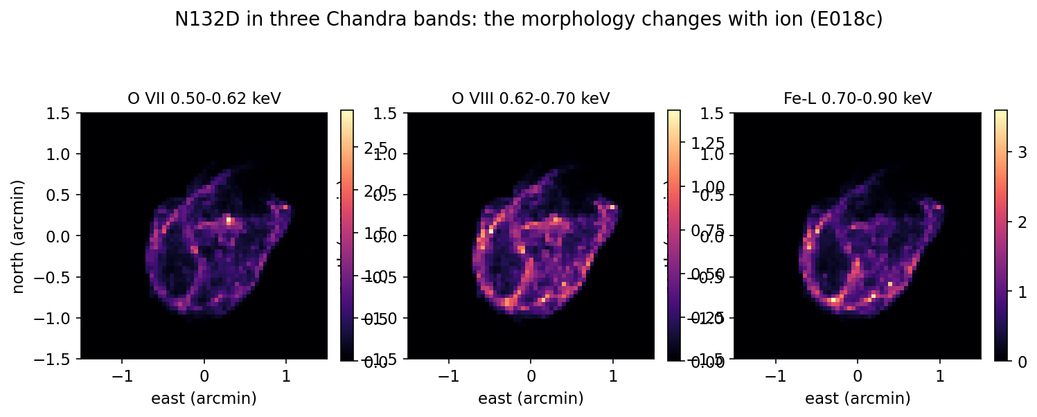
来源:/u/Lang3/Data/S2Fitting/verification/n132d-chandra-bands-20261015-hermes/(E018c 冻结产品:三个波段的 bsub-flux 图与 band_leakage.json);I023 见 cognition-os/03_TRUST_TABLE.md I023 行(Trusted 事实 / Provisional 模板推论)。Source: /u/Lang3/Data/S2Fitting/verification/n132d-chandra-bands-20261015-hermes/ (the frozen E018c products: the bsub-flux images of the three bands and band_leakage.json); I023 is cognition-os/03_TRUST_TABLE.md row I023 (Trusted facts, Provisional template implication).
6.2 算一个数:真实数据长什么样A worked number: what the real data look like
三个观测、每个三条条带的真实 O VII 计数(TOTAL 源计数加缩放背景,E015 冻结包):The real O VII counts of the three observations, each with three strips (TOTAL source counts plus scaled background, the frozen E015 pack):
| 观测Observation | 下条带lower strip | 中央条带central strip | 上条带upper strip |
|---|---|---|---|
| 0210681301 (O1) | 763 | 1325 | 620 |
| 0125100201 (O2) | 3060 | 6095 | 2149 |
| 0811012401 (O3) | 3295 | 12428 | 6481 |
中央条带最亮(N132D 中心落在那里),三个观测的条带计数比互不相同——因为三个观测的 roll 角不同,同一条天空条带投影到不同的条带上。这正是多 roll 的价值:不同投影角度把空间分布与速度场解耦。The central strip is brightest (N132D's centre lands there), and the strip count ratios differ between observations, because the three observations have different roll angles, so the same sky strip projects onto different detector strips. That is the value of multiple rolls: different projection angles decouple the spatial distribution from the velocity field.
来源:/u/Lang3/Data/S2Fitting/verification/n132d-velfield-inputs-20261014/pack_{0210681301,0125100201,0811012401}.npz(source_counts 与 background_counts,2026-10-19 由 make_figures.py 读出并打印)。Source: /u/Lang3/Data/S2Fitting/verification/n132d-velfield-inputs-20261014/pack_{0210681301,0125100201,0811012401}.npz (source_counts and background_counts, read and printed by make_figures.py on 2026-10-19).
7. 讨厌参数7. Nuisance parameters
7.1 概念The concept
讨厌参数(nuisance parameter)是物理上不感兴趣、但必须放进拟合里否则会偏置物理量的量。项目的仪器讨厌参数组(E 组)有四类:A nuisance parameter is a quantity we do not care about physically but must include in the fit, or the physical quantities become biased. The project's instrument nuisance set (set E) has four members:
- \(\delta X_o\):每个观测一个交叉色散偏移。I021 发现前向模型把 N132D 放偏了 \(-6.25 \pm 0.49\)″(探测器坐标);不拟掉它,速度场就带偏。\(\delta X_o\), one cross-dispersion offset per observation. I021 found the forward model misplaces N132D by \(-6.25 \pm 0.49\) arcsec (detector frame); not fitting it biases the velocity field.
- \(w\):一个共同的交叉色散尺度。E018a 发现数据偏好 \(w \approx -3\,\%\);它是什么至今未解(RT14、RT19 都没能解释),但拟掉它代价只有 0.4 % 精度。\(w\), one common cross-dispersion scale. E018a found the data prefer \(w \approx -3\,\%\); what it absorbs is still unexplained (RT14 and RT19 both failed to explain it), but fitting it costs only 0.4 % precision.
- \(f\):线翼比例,带标定源先验。\(f\), a wing fraction with a calibrator prior.
- \(a\):条带外接受度标度(串扰)。\(a\), an out-of-strip acceptance scale (cross-talk).
红队 RT15 检验了这套讨厌参数不会与 \(\sigma_v\) 简并:同时放开全部四个,速度参数的 Fisher 误差只增大 2.4 %(\(\sigma_v\) 57.7 到 59.0 km/s),相关系数只有 \(-0.12\) 与 \(+0.02\)。RT17 又用 16 种形状不同的误差注入检验,其中 15 种的偏差保持在 0.2 SD 以内。Red team RT15 verified that this nuisance set is not degenerate with \(\sigma_v\): freeing all four at once raises the velocity parameters' Fisher error by only 2.4 % (\(\sigma_v\) 57.7 to 59.0 km/s), with correlations of only \(-0.12\) and \(+0.02\). RT17 then injected 16 error shapes that differ from every fitted nuisance; of those, 15 keep the bias within 0.2 SD.
来源:偏移量级取自 I021(\(-6.25 \pm 0.49\)″,Trusted,范围已收窄);伪速度按本页多普勒公式 0.0074 Å 对应 100 km/s 换算;动画为示意,非科学证据。Source: the offset scale comes from I021 (\(-6.25 \pm 0.49\) arcsec, Trusted, narrowed scope); the spurious velocity uses this page's Doppler conversion, 0.0074 Angstrom for 100 km/s; the animation is an illustration, not scientific evidence.
7.2 算一个数:讨厌参数的代价A worked number: the cost of the nuisances
\[ \frac{59.0 - 57.7}{57.7} = 2.3\,\% \]\[ \frac{59.0 - 57.7}{57.7} = 2.3\,\% \]
用 2.3 % 的统计精度换掉一整类未知仪器误差,这是项目最重要的设计决定之一(E018b 的 D0/F/A/E 配置族)。Trading 2.3 % of statistical precision to remove a whole class of unknown instrument errors is one of the project's key design decisions (the D0/F/A/E configuration family of E018b).
来源:cognition-os/03_TRUST_TABLE.md(I021、I025、E018b design RT15、E018b design RT17 行);cognition-os/insights/I029_n132d-ovii-velocity-stage1.md(E 组讨厌参数跑到不物理值的警告)。Source: cognition-os/03_TRUST_TABLE.md (rows I021, I025, E018b design RT15, E018b design RT17); cognition-os/insights/I029_n132d-ovii-velocity-stage1.md (the warning that set E's nuisances run to unphysical values).
8. Fisher 误差与轮廓似然8. Fisher errors and the profile likelihood
8.1 概念The concept
拟合得到最优点 \(\hat{\theta}\) 后,误差从哪来?Fisher 误差(Fisher standard deviation)用似然面的曲率:在 \(\hat{\theta}\) 处算二阶导数矩阵(Hessian),取逆,对角线的平方根就是每个参数的 \(1\sigma\) 误差。它快,但假设似然面是抛物面(参数远离边界、模型正确)。Once the fit finds the optimum \(\hat{\theta}\), where do the errors come from? The Fisher standard deviation uses the curvature of the likelihood surface: compute the matrix of second derivatives (the Hessian) at \(\hat{\theta}\), invert it, and the square roots of the diagonal are the 1-sigma errors. It is fast, but it assumes the likelihood surface is a paraboloid (parameters far from bounds, model correct).
轮廓似然(profile likelihood)更稳健:固定某个参数 \(\theta_j\) 在一系列值上,每次重新优化其余所有参数,记录最小 \(C\)。\(C(\theta_j)\) 曲线上升 \(\Delta C = 1\) 的范围就是 68 % 置信区间(嵌套模型、1 个自由参数)。它慢(每个点一次完整拟合)但不依赖抛物面假设。The profile likelihood is more robust: fix a parameter \(\theta_j\) at a series of values, re-optimise all the others each time, and record the minimum \(C\). The range where the \(C(\theta_j)\) curve rises by \(\Delta C = 1\) is the 68 % confidence interval (nested models, one free parameter). It is slow (a full fit per point) but does not assume a paraboloid.
项目两种都用:Fisher SD 用于红队的“0.2 SD”类结论(快、可比),轮廓似然用于 I029 的括号区间(如 \(\sigma_v = 500 \pm 27\) [470, 530] km/s,前者是 Fisher、后者是 profile 68 %)。The project uses both: Fisher SDs for the red teams' "0.2 SD" style results (fast, comparable), and the profile likelihood for I029's bracketed intervals (e.g. \(\sigma_v = 500 \pm 27\) with profile [470, 530] km/s; the first is Fisher, the second profile 68 %).
8.2 算一个数:梯度到底有多显著A worked number: how significant is the gradient
I029 的 E 组拟合给出 \(|g| = 68 \pm 31\) km/s/′(Fisher)。它的显著性:The set-E fit of I029 gives \(|g| = 68 \pm 31\) km/s per arcmin (Fisher). Its significance:
\[ \frac{|g|}{\mathrm{SD}} = \frac{68}{31} = 2.2\ \text{(Fisher)}, \qquad \text{计入拟合不好后} \approx 1.7\text{–}1.9\sigma \]\[ \frac{|g|}{\mathrm{SD}} = \frac{68}{31} = 2.2\ \text{(Fisher)}, \qquad \text{after inflating for the poor fit} \approx 1.7\text{–}1.9\sigma \]
所以“向西的梯度”只有约 \(1.9\sigma\),而且方向随谱线形状模型变化(L 与 C2 模型差 46°)——项目把它写为“不稳健”,而不是“测到了梯度”。So the "westward gradient" is only about 1.9 sigma, and its direction moves with the line-shape model (46 degrees between the L and C2 models); the project writes "not robust", not "a gradient was measured".
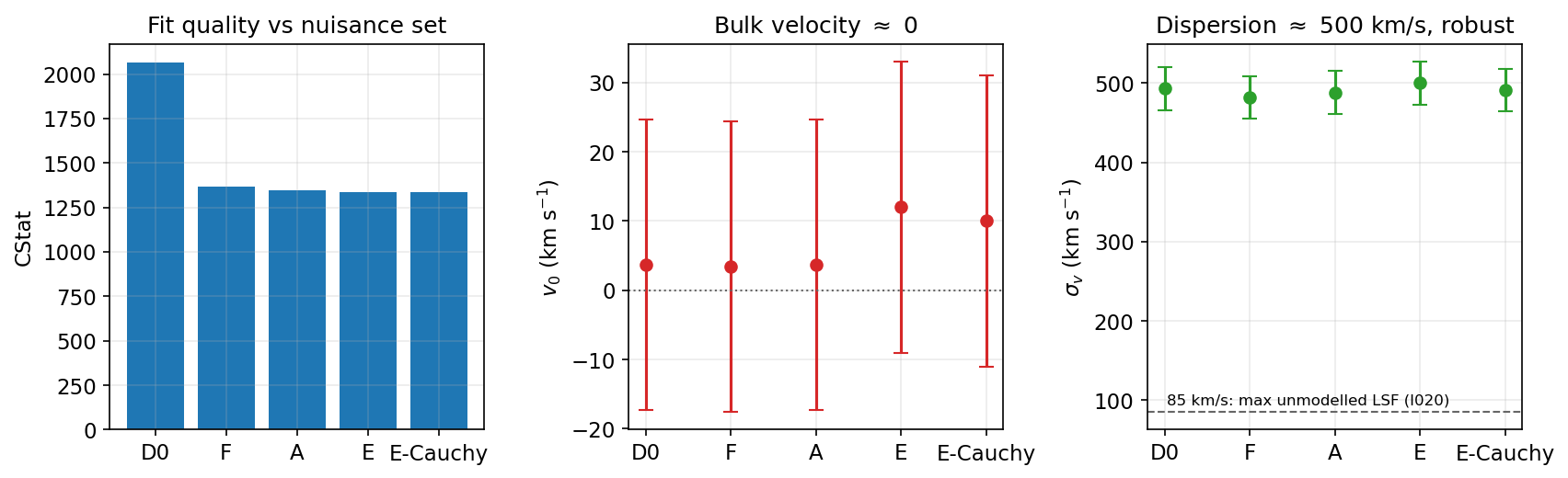
来源:cognition-os/insights/I029_n132d-ovii-velocity-stage1.md(测量表:D0/F/A/E/E-Cauchy 的 CStat、\(v_0\)、\(|g|\)、\(\sigma_v\);Provisional,2026-10-19 修订)。85 km/s 上限来自 I020(Trusted)。Source: cognition-os/insights/I029_n132d-ovii-velocity-stage1.md (the measurement table: CStat, \(v_0\), \(|g|\), \(\sigma_v\) for D0/F/A/E/E-Cauchy; Provisional, amended 2026-10-19). The 85 km/s limit is from I020 (Trusted).