用三个滚转角的 RGS 前向建模，把展源的空间展宽从视向速度场中分离出来Forward modelling three RGS roll angles separates an extended source's spatial broadening from its velocity field

各位好，谢谢介绍。今天讲我们最近的一个方法工作，问题是这样的：怎样用同一台仪器、同一个目标的多次档案观测，把一个延展源的速度场测出来。目标天体是 N132D，大麦哲伦云里一个年轻的超新星遗迹，年龄大约两千五百年，角直径大约三个角分。我会先讲为什么这个问题难——难在仪器把空间和波长混在了一起；再讲我们怎么做——核心是三个不同滚转角的前向建模；最后给出现在测到了什么、还不能说什么。全程 45 分钟，最后留 10 到 15 分钟提问。如果中间有问题，也欢迎随时打断。 如果最后还有时间，我会用备份页讲数据约简的细节和标定源审计的数值。Good afternoon, and thank you for the introduction. Today I will talk about a method we have been developing, and the question is this: how do you measure the velocity field of an extended source using repeated archival observations of one target with one instrument? The target is N132D, a young supernova remnant in the Large Magellanic Cloud, roughly two and a half thousand years old and about three arcminutes across. I will start with why the problem is hard, and it is hard because the instrument mixes space and wavelength together. Then I will explain how we approach it, where the core idea is forward modelling at three different roll angles. I will finish with what we have measured and what we still cannot claim. The talk is forty-five minutes, with ten to fifteen minutes for questions at the end. Please feel free to interrupt in the middle as well if something is unclear. If there is time at the end I will use the backup pages for the data-reduction details and the calibrator-audit numbers.

累计 1:51。Cumulative 1:51.

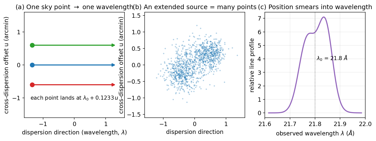
先说问题本身。对点源，光谱线的宽度就是物理：热运动、湍流、整体膨胀——线宽直接给出速度弥散。但对一个跨几个角分的延展源，用无狭缝光栅光谱仪——XMM-Newton 的 RGS——测到的线宽里还混着第三样东西：源的角延展。请看图：仪器把天空位置直接映射到波长上，源的一端和另一端发出的同一条线，落在不同的波长通道里。于是"线宽"不再是一个物理量，而是物理速度、源的形状和仪器响应三者的卷积。这不是 N132D 特有的困难，是所有用 RGS 看展源的人共同面对的困难。今天要讲的，就是把这三者分开。为什么值得做？因为速度场是连接爆炸机制与当前动力学状态的直接证据：它记录激波往哪推进、喷出物怎么分布、周际介质有没有密度梯度。没有速度场，我们只能看到一张静态照片。 顺带说一句，这个困难在光学波段也有——只是那里的仪器有狭缝，或者有像面尺寸，所以不明显。 这个困难的定量版本是：一个 3 角分的源，它的线宽里有一半以上来自几何而不是速度。Let me start with the problem itself. For a point source, a spectral line's width is physical: thermal motion, turbulence, bulk expansion — the width directly gives the velocity dispersion. But for an extended source spanning several arcminutes, measured with a slitless grating spectrometer — XMM-Newton's RGS — the width contains a third ingredient: the source's angular extent. Look at the figure: the instrument maps sky position directly onto wavelength, so the same line emitted at the two ends of the source lands in different wavelength channels. So "line width" is no longer one physical quantity but a convolution of physical velocities, the source's shape and the instrument response. This is not a difficulty peculiar to N132D; it is the shared difficulty of everyone who looks at extended sources with the RGS. Separating these three is what this talk is about. And why is it worth doing? Because the velocity field is the direct evidence connecting the explosion mechanism to the present dynamics: it records where the shock is advancing, how the ejecta are distributed, and whether the circumstellar medium has density gradients. Without a velocity field we have only a static photograph. The same difficulty exists at optical wavelengths, incidentally; it is just less visible there because those instruments have a slit, or a detector format, that separates the two. The quantitative version of the difficulty: for a source 3 arcminutes across, more than half of its line width comes from geometry rather than velocity.

累计 3:43。Cumulative 3:43.

这是今天的路线。第一部分背景，四分钟；第二部分数据与方法，十分钟；第三部分三个结论，十五分钟；第四部分系统误差与诚实的限制，八分钟；第五部分下一步与总结，六分钟。我承诺两件事。第一，你会看到一个可复现的测量是怎么一步一步建起来的：每一步怎么验、验的阈值是多少、失败过什么。第二，我会明确区分什么是测稳了的、什么还只是初步——今天最重要的三个数里有两个带"初步"标签，我会说清楚为什么。还有一件事我事先说明：如果某个问题我今天答不了，我会直接说不知道，而不是给一个听起来合理的答案。这个项目里"待定"是一个正式的结论状态，不是一个回避。现在开始第一部分。 还有一点：今天讲的都是 2026-10-19 之前已记录的结论；在那之后的新结果，等它们通过复核再讲。Here is the route. Part one is background, four minutes; part two is data and method, ten minutes; part three is the three findings, fifteen minutes; part four is systematics and honest limitations, eight minutes; part five is next steps and the summary, six minutes. I promise two things. First, you will see how a reproducible measurement is built step by step: how each step is verified, what the acceptance thresholds are, and what has failed along the way. Second, I will be explicit about what is robust and what is still preliminary — two of the three headline numbers today carry a preliminary label, and I will explain exactly why. One more thing I should say up front: if there is a question I cannot answer today, I will say I do not know, rather than give an answer that merely sounds plausible. In this project "pending" is a formal conclusion state, not an evasion. Now, part one. One more point: everything I present today was recorded before 2026-10-19; newer results wait until they pass review.

累计 5:05。Cumulative 5:05.

第一部分是背景，四张幻灯片：RGS 是什么、它的色散定律是什么、N132D 是什么、以及为什么"线宽"这个量对延展源会失效。这一部分不需要任何 X 射线光谱的专业背景，我会从零讲起。这里先交代一个术语习惯，后面会反复用：色散方向，指波长展开的方向；交叉色散方向，指与它垂直、对应天空位置的方向。RGS 抽谱是在交叉色散方向上取矩形条带，所以"条带"就是一小片天空。整个方法的所有困难都来自一个事实：这两个方向在仪器里被绑在一起。如果记不住别的，请记住下一张幻灯片上的那个换算——每一角分的交叉色散等于 1690 km/s。 另外，今天所有速度都相对大麦哲伦云静止系，这是本项目约定的参考系。Part one is background, four slides: what the RGS is, what its dispersion law is, what N132D is, and why "line width" fails as a quantity for an extended source. No specialist background in X-ray spectroscopy is needed for this part; I will build it up from zero. Let me fix one pair of terms first, because I will use them repeatedly. The dispersion direction is the one along which wavelength is spread out. The cross-dispersion direction is perpendicular to it and maps sky position. RGS extraction takes rectangular strips along the cross-dispersion direction, so a "strip" is simply a small piece of sky. Every difficulty in this method comes from one fact: these two directions are tied together inside the instrument. If you remember nothing else, remember the conversion on the next slide — one arcminute of cross-dispersion equals 1690 km/s. Also, all velocities today are relative to the Large Magellanic Cloud rest frame, the reference frame this project adopts by convention.

累计 6:20。Cumulative 6:20.

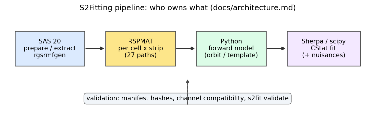
RGS，反射光栅光谱仪，是 XMM-Newton 上的两台高分辨率光谱仪。它没有入射狭缝：光子按波长沿色散方向偏折，而垂直方向——交叉色散——直接对应天空位置。对点源，交叉色散位置固定，波长轴干净。它的能量分辨率极高：在 21.8 Å 附近，仪器线扩散函数的等效速度宽度只有约 437 km/s。这个数很重要，后面会拿它当尺子：任何未建模的仪器展宽必须远小于它，否则测出来的弥散就不可信。代价是没有空间分辨——这是它和 Chandra 的根本区别。图上是整个项目的管线骨架：SAS 负责校准、事件与抽谱；逐源位置响应矩阵把天空模板折成期望计数；Python 与 Sherpa 做前向模型与拟合。今天的报告只涉及右半边——拿到抽谱之后，前向模型怎么建、怎么拟。左半边是数据约简，备份页 B1 有细节。请注意中间那个"27 条路径"：9 个源格各映射到 3 条带，这是展源算子相对点源多出来的工作量。 RGS 有两台，RGS1 与 RGS2；本报告的速度测量用 RGS1，因为它的有效面积在 O VII 波段更大。The RGS, the Reflection Grating Spectrometer, is the pair of high-resolution spectrometers on XMM-Newton. It has no entrance slit: photons are deflected by wavelength along the dispersion direction, while the perpendicular direction, the cross-dispersion, maps sky position directly. For a point source the cross-dispersion position is fixed and the wavelength axis is clean. Its energy resolution is superb: near 21.8 Angstrom the line-spread function is equivalent to only about 437 km/s. That number matters, and we will use it as a yardstick later: any unmodelled instrumental broadening must be far below it, or the measured dispersion is not credible. The price is that it has no spatial resolution — that is the fundamental difference from Chandra. The figure shows the whole project's pipeline skeleton: SAS owns calibration, events and extraction; per-position response matrices fold a sky template into expected counts; Python and Sherpa do the forward model and the fit. Today's talk concerns only the right half — once the spectra are extracted, how the forward model is built and fitted. The left half is data reduction, and backup page B1 has the details. Note the "27 paths" in the middle: 9 source cells each mapping to 3 strips, which is the extra work the extended-source operator demands compared with a point source. There are two of them, RGS1 and RGS2; the velocity measurement in this talk uses RGS1, because its effective area is larger in the O VII band.

累计 8:10。Cumulative 8:10.

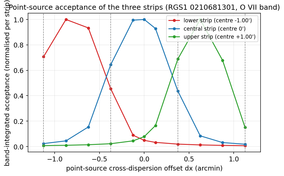
这条曲线是全部工作的基础，值得看仔细。横轴是点源相对条带中心的交叉色散偏移，纵轴是落进条带的响应。三条曲线是三条条带，各 0.75 角分宽，中心在负 0.75、0 和正 0.75 角分；竖直虚线是条带的几何边界。两个事实。第一，每条带只接受邻近天空，但两侧有翼，延伸到约 1.25 角分——所以条带计数里混着带外的光，项目把这叫串扰；后面会看到这是讨厌参数组的一个成员。要说明的是：这不是仪器缺陷，是光栅的物理散射，任何条带式抽谱都有它，只是多数工作不需要在意。第二，把这些曲线和色散定律放在一起，就得到关键的换算：交叉色散每偏一个角分，谱线移动 0.1233 Å；在 21.8 Å 处，这等于每角分约 1690 km/s。请记住这个数，后面所有系统误差都拿它当尺子。这个换算不是我们测的唯一来源——三个观测一致给出 0.1236 到 0.1238 Å 每角分——但它是冻结输入包里用的值。 顺便说，这三条曲线也是我们后面所有模拟检验的输入，不是从文献抄来的。This curve is the foundation of the whole work, and it rewards a careful look. The horizontal axis is a point source's cross-dispersion offset from the strip centre, the vertical axis the acceptance into the strip. The three curves are the three strips, each 0.75 arcmin wide, centred at minus 0.75, zero and plus 0.75 arcmin; the vertical dashed lines are the strips' geometric boundaries. Two facts. First, each strip accepts only nearby sky, but with wings reaching about 1.25 arcmin either side, so strip counts contain light from outside the strip; the project calls this cross-talk, and you will see it is one member of the nuisance set. To be clear: this is not an instrument defect but the grating's physical scattering, and any strip-based extraction has it — most work just never needs to care. Second, put these curves together with the dispersion law and you get the key conversion: each arcminute of cross-dispersion moves a line by 0.1233 Angstrom, which at 21.8 Angstrom is about 1690 km/s per arcminute. Please remember that number: every systematic later in this talk is measured against it. This conversion is not the only measurement — the three observations consistently give 0.1236 to 0.1238 Angstrom per arcmin — but it is the value used in the frozen input packs. Incidentally, these three curves are also the input to every simulation test later in this project; they are not taken from the literature.

累计 10:00。Cumulative 10:00.

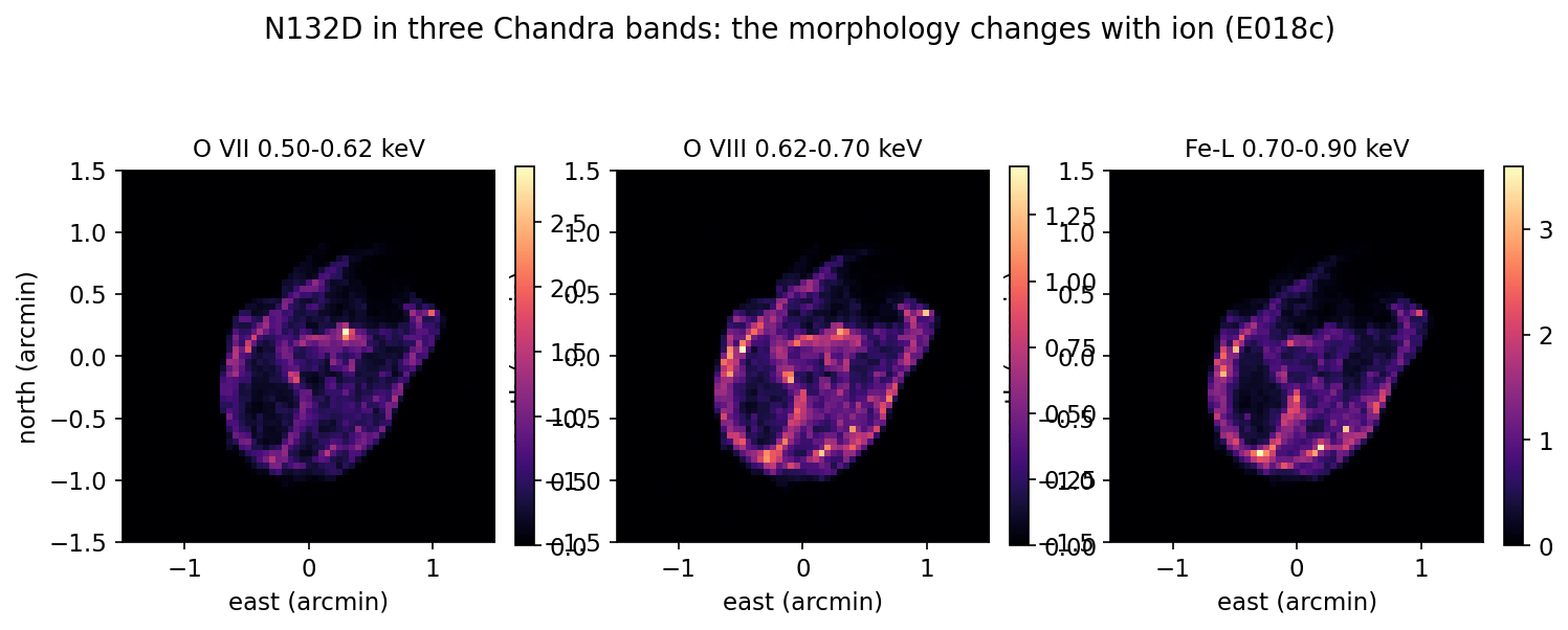
目标天体 N132D，大麦哲伦云里最亮的 X 射线超新星遗迹之一，年龄约 2500 年，角直径约 3 角分。3 角分对 RGS 来说足够延展：按色散定律，3 角分就是 0.37 Å，在 21.8 Å 处折合约 5000 km/s 的表观展宽。所以这个源的线宽完全被几何支配。图上是 Chandra 三个波段的像，横轴东向、纵轴北向，都是角分。可以清楚看到形态随电离阶段改变：O VII、O VIII 与 Fe-L 三个波段的空间分布不同。这既是机会——不同线看不同气体——也是风险：用一个天空模板描述三条谱线未必成立。请注意东北方向的 breakout 结构和外层的马蹄形，这是文献里描述过的几何。请记住这张图，第四部分会回到它：这正是当前最大系统误差的来源。 这个源的年龄意味着激波仍在加速，所以速度场是动力学状态的直接读数。The target, N132D, is among the brightest X-ray supernova remnants in the Large Magellanic Cloud, about 2500 years old and about 3 arcminutes across. Three arcminutes is extended enough for the RGS: by the dispersion law, 3 arcminutes is 0.37 Angstrom, about 5000 km/s of apparent broadening at 21.8 Angstrom. So this source's line width is dominated entirely by geometry. The figure shows Chandra images in three bands, east horizontal and north vertical, both in arcminutes. You can clearly see the morphology change with ionisation stage: the O VII, O VIII and Fe-L bands have different spatial distributions. That is both an opportunity — different lines see different gas — and a risk: one sky template may not describe all three lines. Note the breakout structure toward the northeast and the outer horseshoe, a geometry described in the literature. Keep this figure in mind; part four returns to it, because it is the source of the largest current systematic. The source's age means the shock is still accelerating, so the velocity field is a direct readout of the dynamical state.

累计 11:23。Cumulative 11:23.

这张幻灯片是动态的，我们按播放看一遍。左边竖轴是天空的交叉色散位置，右边横轴是探测器上的波长。按播放，一个天空点沿着色散方向逐帧移动；每到一个位置，它发出的光就按色散定律落到右边对应的波长上，这些蓝色短线就是光子走过的路径。右边这些紫色点是累积起来的谱线轮廓——随着天空点扫过整个源，轮廓一点点长出来。要点在这里：轮廓的形状就是天空亮度分布的复制，只是横轴换成了波长。所以"线宽"里有多少是几何、多少是速度，单看一条光谱分不出来。这正是要三个滚转角的原因。动画用的是示意性的三团亮度，不是真实数据；真实数据在下一页的表里。 动画的控制按钮在下面：播放、单步、复位；动画字符串跟随页面语言切换。This slide is animated, so let us press play and watch it once. The vertical axis on the left is the sky's cross-dispersion position, the horizontal axis on the right is wavelength on the detector. Press play and one sky point advances along the dispersion direction frame by frame; at each position its light lands on the right at the wavelength the dispersion law assigns, and these short blue lines are the paths the photons take. The purple points on the right are the accumulating line profile — as the sky point sweeps across the source, the profile grows bit by bit. Here is the point: the profile's shape is a copy of the sky brightness distribution, with the horizontal axis relabelled as wavelength. So how much of the "line width" is geometry and how much is velocity cannot be separated from one spectrum alone. That is exactly why three roll angles are needed. The animation uses three illustrative brightness clumps, not real data; the real data are in the table on the next page. The animation's controls are below it: play, step and reset, and its strings follow the page language.

累计 12:51。Cumulative 12:51.

第二部分讲我们怎么做。核心是一个决定：不去反演，而是前向建模。反演的思路是"从观测反推天空"，听起来直接，但 RGS 的混合是高度退化的——一条光谱对应一整片天空，方程远少于未知数——反演会把噪声放大成假结构。前向建模反过来：把天空模板、速度场、仪器算子串成期望计数，直接和观测比，然后调参数让两者一致。代价是每一步都要显式建模，好处是每一个假设都摆在明面上、都可以单独检验；一个假设错了，你能指出是哪一步错了。这一部分四张幻灯片：数据、前向模型、讨厌参数组、以及一个动画说明为什么讨厌参数不可省。另外交代一句统计框架：我们用 Cash 统计量，也就是泊松似然的负两倍，不用卡方——因为每条通道只有几个计数，高斯近似不成立。 这一部分也交代一个边界：我们只做速度场，不做等离子体诊断——那需要更宽的波段和更完整的谱线清单。Part two is how we do it. The core decision: no inversion, but forward modelling. Inversion says "work backwards from the observation to the sky", which sounds direct, but the RGS mixing is highly degenerate — one spectrum corresponds to a whole piece of sky, so there are far fewer equations than unknowns — and inversion amplifies noise into spurious structure. Forward modelling goes the other way: chain the sky template, the velocity field and the instrument operator into expected counts, compare directly with the observation, and adjust the parameters until they agree. The cost is that every step must be modelled explicitly; the benefit is that every assumption is on the table and can be tested on its own, and if an assumption is wrong you can say which step it is. Four slides in this part: the data, the forward model, the nuisance set, and an animation showing why the nuisance set is not optional. One more note on the statistical framework: we use the Cash statistic, minus twice the Poisson log-likelihood, not chi-squared, because each channel holds only a few counts and the Gaussian approximation does not hold. One boundary to state in this part: we do only the velocity field, not plasma diagnostics, which would need a wider band and a complete line list.

累计 14:30。Cumulative 14:30.

数据是三样东西。第一，N132D 的三个 RGS 观测，滚转角大约 0、90、180 度——三个近似正交的方向，这是整个方法能成立的关键。为什么关键？因为一个滚转角只能把天空沿一个方向投影到波长上；三个近正交的方向给出同一速度场的三个投影，联立才能解耦空间与速度。用一个比喻：从三个方向拍同一个物体的影子，才能重建物体本身；只从一个方向拍，影子和物体不可分。第二，一个 Chandra 档案观测，提供天空模板：我们需要知道源在天空上长什么样。第三，一批标定源观测，用来审计仪器。表上是三个科学观测与它们的 O VII 波段计数，合计约 3.3 万。计数不多，所以后面会看到统计误差是主要限制之一。天空模板来自 Chandra 的 0.50 到 0.62 keV 波段，重采样到 0.05 角分网格——这个波段不纯净，第四部分会讲污染有多大。三个观测的计数差别很大，最暗的只有 2708 个计数，这会进入最终的权重。 三个观测的曝光不同、计数不同，联合拟合并不会因此偏袒最亮的那个，因为泊松似然自己按计数加权。The data are three things. First, three RGS observations of N132D at roll angles of roughly 0, 90 and 180 degrees — three near-orthogonal directions, which is what makes the whole method work. Why does it matter? Because one roll angle projects the sky onto wavelength along only one direction; three near-orthogonal directions give three projections of one velocity field, and fitting them jointly is what decouples space from velocity. An analogy: you need shadows photographed from three directions to reconstruct an object; from one direction alone, shadow and object are inseparable. Second, one archival Chandra observation, which supplies the sky template: we need to know what the source looks like on the sky. Third, a set of calibrator observations, used to audit the instrument. The table lists the three science observations and their O VII-band counts, about 3.3 x 10^4 in total. That is not a lot of counts, so the statistical error will be one of the main limits. The sky template comes from the Chandra 0.50-0.62 keV band resampled onto a 0.05 arcmin grid — that band is not pure, and part four covers how large the contamination is. The three observations differ a lot in counts, the faintest having only 2708, and that feeds into the final weighting. The three observations have different exposures and counts, and the joint fit does not favour the brightest one, because the Poisson likelihood weights by counts itself.

累计 16:20。Cumulative 16:20.

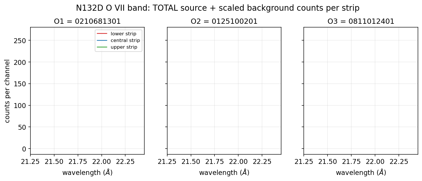
前向模型四步。第一，天空模板：Chandra 像给出每个天空像素的相对亮度。第二，速度场：每个像素一个视向速度，我们参数化为一个平面场——零点加一个梯度——再叠加一个高斯弥散。第三步和第四步的顺序是全部关键：第三，谱线模型，O VII 三重线三条独立振幅加一个连续谱，谱线先被速度场移动；第四，仪器算子，把每个像素的光按探针响应折成每条条带的期望计数，也就是被色散几何摊开，再乘曝光剖面、加缩放背景。然后把三个观测、九条条带谱联立，最小化 Cash 统计量——泊松似然的负两倍。图上就是拟合对象：三个观测的 O VII 波段谱，横轴波长从 21.25 到 22.45 Å，纵轴每通道计数，三条曲线是三条条带。请留意三条谱线的位置与宽度随观测而变，因为天空结构投影到色散几何的方式随滚转角改变——这正是多滚转方法利用的信息。 误差报两种：Fisher 标准差，来自似然面在极小值处的曲率；以及轮廓似然区间，固定一个参数、重新优化其余。两者在本例中接近，我们报 Fisher 的那个。 这个模型的可检验性来自它的显式性：如果结论错了，我们能指出是哪一步的假设错了。The forward model has four steps. First, the sky template: the Chandra image gives each sky pixel's relative brightness. Second, the velocity field: one line-of-sight velocity per pixel, which we parametrise as a plane field — a zero point plus a gradient — with one Gaussian dispersion on top. The order of steps three and four is the whole key: third, the line model, three independent amplitudes for the O VII triplet plus a continuum, where the lines are first shifted by the velocity field; fourth, the instrument operator, which folds each pixel's light through the probe responses into expected counts per strip, that is, spreads it with the dispersion geometry, then multiplies by the exposure profile and adds the scaled background. The Cash statistic — minus twice the Poisson log-likelihood — is then minimised jointly over three observations and nine strip spectra. The figure is what we fit: the O VII-band spectra of the three observations, wavelength from 21.25 to 22.45 Angstrom horizontal, counts per channel vertical, the three curves being the three strips. Notice that the lines' positions and widths change from observation to observation, because how sky structure projects onto the dispersion geometry changes with the roll angle — and that is exactly the information the multi-roll method exploits. We report two kinds of error: the Fisher standard deviation, from the curvature of the likelihood surface at the minimum, and the profile-likelihood interval, obtained by fixing one parameter and re-optimising the rest. In this case they agree closely, and we quote the Fisher one. The model's testability comes from its explicitness: if a conclusion is wrong, we can point to which step's assumption was wrong.

累计 18:26。Cumulative 18:26.

讨厌参数组是本项目最重要的设计决定。四个成员，每一个都有标定源或注入检验作为依据，不是凭空加的。第一个，每个观测一个交叉色散偏移：前向模型把 N132D 放偏了 6.25 角秒，所以每个观测需要一个自由偏移把它挪回来。第二个，一个共同的交叉色散尺度：数据偏好约负 3 %，成因至今未解，后面会讲。第三个，线翼比例，带标定源先验。第四个，条带外接受度标度，处理刚才说的串扰——条带计数有 14 到 38 % 来自带外。现在算代价：同时放开四个，速度弥散的 Fisher 误差从 57.7 增到 59.0 km/s，2.4 %；与速度弥散的相关系数不超过 0.12。用 2.4 % 的统计精度换掉一整类未知仪器误差，这是我们做过的最划算的交易。为什么划算？看下一个动画。 顺便回答一个常见问题：为什么不用更少的参数？因为省下的那 2.4 % 换不回一整类未知误差，账算不过来。 四个参数的共同点是：它们描述的都是仪器的几何，不是天空的物理。The nuisance set is this project's most important design decision. Four members, each resting on calibrator data or an injection test, none added on a hunch. First, one cross-dispersion offset per observation: the forward model misplaces N132D by 6.25 arcsec, so each observation needs a free offset to move it back. Second, one common cross-dispersion scale: the data prefer about minus 3 %, and its cause is still unexplained, as I will discuss later. Third, a wing fraction with a calibrator prior. Fourth, an out-of-strip acceptance scale, which handles the cross-talk I mentioned: 14 to 38 % of strip counts come from outside the strip. Now the cost: freeing all four raises the velocity dispersion's Fisher error from 57.7 to 59.0 km/s, that is 2.4 %, with correlations with the dispersion below 0.12. Trading 2.4 % of statistical precision to remove a whole class of unknown instrument error is the best deal we made. Why is it a deal? See the next animation. This also answers a question people often ask: why not use fewer parameters? Because the 2.4 % saved does not buy back a whole class of unknown error, and the arithmetic does not work. What the four parameters have in common is that they all describe the instrument's geometry, not the sky's physics.

累计 20:04。Cumulative 20:04.

为什么必须拟掉偏移，这个动画把账算清楚。交叉色散移动 0.06 角分——约 3.6 角秒，一个 XDSP 像素量级——带来的色散移动是 0.0074 Å。同一页的多普勒公式说，0.0074 Å 在 21.8 Å 处对应 100 km/s。两个数几乎相等。所以一个像素的空间错位，就能让整条谱线移动，看起来完全像一个速度。按播放：红色虚线是带偏移的观测，绿色是真实速度，蓝色是拟掉偏移后的恢复，右下角标出当前偏移对应的伪速度。请注意恢复曲线和真实曲线几乎重合——这就是那 2.4 % 买回来的东西。不拟，速度场不可信；拟了，代价只有 2.4 %。这就是四个参数存在的全部理由。动画是示意，不是科学证据；偏移量级取自前向模型的实测放偏。 还要说清楚这个动画的边界：它演示的是一个偏移如何伪装成速度，不是我们的拟合过程本身。Why the offset must be fitted out — this animation does the arithmetic. A cross-dispersion shift of 0.06 arcmin, about 3.6 arcsec or of order one XDSP pixel, moves the line by 0.0074 Angstrom. The Doppler formula on the same page says 0.0074 Angstrom at 21.8 Angstrom is 100 km/s. The two numbers are almost equal. So a one-pixel spatial misplacement shifts the whole line and looks exactly like a velocity. Press play: the dashed red line is the offset observation, green is the true velocity, blue is the recovery after fitting the offset out, and the lower right shows the spurious velocity corresponding to the current offset. Notice that the recovery curve and the true curve nearly coincide — that is what the 2.4 % buys back. Without fitting, the velocity field is not credible; with fitting, the cost is only 2.4 %. That is the entire reason the four parameters exist. The animation is an illustration, not scientific evidence; the offset scale comes from the measured misplacement of the forward model. One boundary to be clear about: this animation shows how an offset masquerades as a velocity; it is not our fitting procedure itself.

累计 21:33。Cumulative 21:33.

第三部分是结果，也是今天最重要的部分。三个结论，每个都有它的证据幻灯片。第一个：弥散约 500 km/s，是真实的物理展宽，不是仪器效应。第二个：气体相对大麦哲伦云静止，速度零点定在一个像素的十分之一尺度上。第三个：梯度只有 1.9 个标准差、方向不稳健，所以只作为上界报告，不作为方向性结论。三个结论加起来回答开头的问题：三个滚转角确实把空间展宽从速度场中分离出来了。请注意，这三个数都是初步结果，第四部分会讲为什么。这里先给一个阅读提示：接下来三张幻灯片，每张的标题就是那张幻灯片要证明的断言，图是证据；如果只看图，请看误差棒和虚线，它们是判断的关键。我们按顺序来。Part three is the results, and the most important part of this talk. Three findings, each with its evidence slide. First: a dispersion of about 500 km/s, which is genuine physical broadening, not an instrumental effect. Second: the gas is at rest in the Large Magellanic Cloud frame, with the velocity zero point pinned to a tenth of a pixel. Third: the gradient is only 1.9 sigma with a non-robust direction, so it is reported as an upper limit only, not as a directional claim. Together the three findings answer the question I opened with: three roll angles do separate the spatial broadening from the velocity field. Note that all three numbers are preliminary, and part four explains why. One reading hint first: over the next three slides, each headline is the assertion that slide proves and the figure is the evidence; if you only look at the figures, look at the error bars and the dashed lines, because they carry the judgement. Let us take them in order.

累计 22:51。Cumulative 22:51.

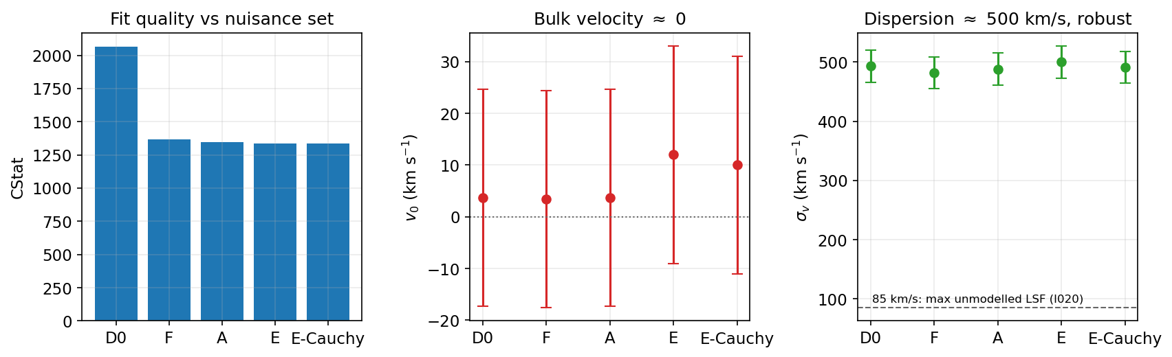
第一个结论，看右图。纵轴是速度弥散，横轴是五种讨厌参数配置，从最简的 D0 到最完整的 E，再加一个柯西替代。五种配置给出一致的弥散，从 482 到 500 km/s——一致性本身就是证据：说明它不是某个参数配置的产物。误差棒是 27 km/s，1 个标准差的 Fisher 误差。水平虚线是 85 km/s，未建模仪器展宽的允许上限。实测值大约是它的六倍。所以这是真实的物理展宽，不是仪器效应。这个数和一个 2500 年历史的超新星遗迹、和 Chandra 像上那些膨胀结的速度，量级上是一致的：氧发射来自快速膨胀的喷出物。左图是拟合质量，Cash 统计量从最简配置的 2065 降到完整配置的 1335——讨厌参数确实在做事。这个结论我今天会重复三次，因为它是最稳的一个。 如果只记今天一个数，请记这个：500 km/s，相对 85 km/s 的仪器上限。 误差棒 27 km/s 是 Fisher 标准差，也就是似然面曲率给出的 1 个标准差。The first finding, look at the right panel. The vertical axis is the velocity dispersion, the horizontal axis the five nuisance configurations, from the simplest D0 to the complete E, plus one Cauchy alternative. The five configurations give a consistent dispersion, from 482 to 500 km/s — and the consistency is itself the evidence: it shows the result is not an artefact of one parameter choice. The error bars are 27 km/s, the one-sigma Fisher error. The dashed horizontal line is 85 km/s, the allowed limit on unmodelled instrumental broadening. The measured value is about six times larger. So this is genuine physical broadening, not an instrumental effect. The number is also consistent, in order of magnitude, with a supernova remnant 2500 years old and with the expansion speeds of the knots in the Chandra image: the oxygen emission comes from fast-expanding ejecta. The left panel is the fit quality: the Cash statistic falls from 2065 for the simplest configuration to 1335 for the complete one, so the nuisance parameters are doing real work. I will repeat this finding three times today, because it is the most robust of the three. If you remember one number from today, remember this one: 500 km/s against the 85 km/s instrumental limit. The 27 km/s error bars are Fisher standard deviations, that is, one sigma from the likelihood surface's curvature.

累计 24:38。Cumulative 24:38.

第二个结论是速度零点：12 正负 21 km/s，相对大麦哲伦云静止系。误差 21 km/s 是什么概念？按色散定律，21 km/s 在 21.8 Å 处只相当于 0.0016 Å，也就是约 0.013 角分的交叉色散偏移。我们能在一个像素的十分之一尺度上定住速度零点，靠的就是三个滚转角互相约束。中图显示五种配置全部落在零附近，误差棒 21 km/s，虚线是零。要强调：这个"零"是一个测量结果，不是一个假设——我们把波长零点完全交给数据，没有加任何外部约束。它也是一个有用的健全性检查：如果三个滚转角的联合拟合有残余系统偏移，这个数不会落在零附近。 这也说明为什么我们不接受「先固定波长零点再拟合速度」这种顺序——那样会把零点变成一个不可检验的假设。 如果速度零点偏离零，那通常意味着波长标定有问题，而不是天体在运动。The second finding is the velocity zero point: 12 plus or minus 21 km/s, relative to the Large Magellanic Cloud rest frame. What does 21 km/s mean? By the dispersion law, 21 km/s at 21.8 Angstrom is only 0.0016 Angstrom, about 0.013 arcmin of cross-dispersion. We pin the velocity zero point to a tenth of a pixel, and that comes from the three roll angles constraining each other. The centre panel shows all five configurations near zero, with 21 km/s error bars and the dotted line at zero. I stress: this "zero" is a measurement, not an assumption — we leave the wavelength zero point entirely to the data, with no external constraint. It is also a useful sanity check: if the joint fit of the three roll angles had a residual systematic offset, this number would not sit near zero. That is also why we do not accept the order of fixing the wavelength zero point first and fitting the velocity afterwards, which would turn the zero point into an untestable assumption. If the velocity zero point were off zero, that would usually mean a wavelength-calibration problem rather than a moving source.

累计 26:09。Cumulative 26:09.

第三个结论是关于梯度的，也是最需要小心的。平面速度梯度拟合给出 68 正负 31 km/s 每 5 角分。68 除以 31，只有 1.9 个标准差——按惯例这不算探测。更麻烦的是方向：换一个先验，方向就转。所以我们不报告方向，只报告幅度上界。O VIII 那一列更糟：拟合优度检验不合格，p 等于 0.005，意思是数据和"单高斯速度分布加当前谱线清单"这个模型对不上。所以 O VIII 的数字只能理解为：在那个速度模型下拟合会给出这些值，而不是 O VIII 的独立结论。我要特别强调这一点，因为这是今天最容易被误读的数：如果有人引用"O VIII 梯度约 111 km/s 每 5 角分"，请同时引用 p 等于 0.005。表上 O VII 的零点那一列我给的是待定，因为第二阶段的细网格会重新定它；弥散和梯度是第一阶段的值。 我预期提问阶段会有关于梯度的问题，备份页 B5 准备了两种解释的细节。 表格里 O VII 与 O VIII 两列并列，是为了显示我们不是只挑好的那一列报。The third finding is about the gradient, and it needs the most care. The planar velocity-gradient fit gives 68 plus or minus 31 km/s per 5 arcminutes. 68 over 31 is only 1.9 sigma — by convention not a detection. Worse, the direction: change the prior and the direction rotates. So we do not report a direction, only a magnitude upper limit. The O VIII column is worse: the goodness-of-fit test fails, p equals 0.005, meaning the data disagree with the model "one Gaussian velocity distribution plus the current line list". So the O VIII numbers mean only: under that velocity model the fit returns these values, not an independent O VIII conclusion. I especially want to stress this, because it is the number most likely to be misread today: if anyone quotes "the O VIII gradient is about 111 km/s per 5 arcminutes", please quote p equals 0.005 with it. In the table I have left the O VII zero point as pending, because the stage-two fine grid will re-determine it; the dispersion and gradient are the stage-one values. I expect questions about the gradient, and backup page B5 has the details of the two readings. The O VII and O VIII columns sit side by side so you can see we are not reporting only the favourable one.

累计 27:51。Cumulative 27:51.

一个自然的怀疑：500 km/s 是不是只是两个相反方向运动的团块平均出来的？换句话说，梯度会不会就是宽度的主要来源？我们做了这个检验：按色散符号把天空分成两半，每半给一个独立的速度偏移，共加四个参数。拟合改善 101，按四个参数算是有意义的。但关键在于：每半自己还需要约 440 km/s 的弥散。换句话说，把最明显的那一个梯度成分拿掉，宽度几乎没变。所以宽度主要是每个局部自己的内部运动，不是大尺度梯度。这个结论比第一个结论更稳健，因为它不依赖速度场的具体形状——不管你把速度场参数化成平面、两半还是别的什么，宽度都还在。这也是我对"弥散 500 km/s"这个结论有信心的第二个理由。 这个检验的设计思想值得记住：与其争论速度场的形状，不如直接检验「宽度是否由梯度贡献」。 四个参数换来的是这个判断，我认为值。A natural suspicion: is 500 km/s just the average of two clumps moving in opposite directions? In other words, could the gradient be the main source of the width? We tested exactly that: split the sky by dispersion sign, give each half its own velocity offset, four extra parameters in total. The fit improves by 101, which is meaningful for four parameters. But the key point: each half still needs about 440 km/s of dispersion on its own. In other words, remove the most obvious gradient component and the width barely changes. So the width is mostly each region's own internal motion, not a large-scale gradient. This conclusion is more robust than the first, because it does not depend on the velocity field's specific shape — whether you parametrise the velocity field as a plane, as two halves, or as something else, the width is still there. That is the second reason I have confidence in the "dispersion of 500 km/s" finding. The design idea here is worth remembering: rather than argue about the velocity field's shape, test directly whether the width is contributed by the gradient. Four parameters buy that judgement, and I think it is worth it.

累计 29:24。Cumulative 29:24.

第四部分是今天最该听的部分：如果这些数不可信，错在哪里。四条：模板系统误差——当前最大的一项，0.3 到 0.6 个标准差；点源响应误差——已量化、已控制，拟掉后不超过 0.05；拟合优度——O VIII 不合格，p 等于 0.005；以及方法本身的方向信息损失——根本性的极限，第二阶段的细网格会量化它。我会给每一条一个数值大小，不给数值的批评不算批评。还要说明这四条之间的关系：前两条是"我们知道自己错了多少"，后两条是"我们不知道自己错了多少"。前者可以报成误差棒，后者只能报成待定。这也是为什么我把 O VIII 那一列标成条件性结果，而把 O VII 的弥散标成初步结果而不是确定结论。 还有一点：这四个限制的大小都给了数值，所以它们是可比较的，不是并列的恐吓。Part four is the part you should listen to most carefully: if these numbers are not to be trusted, where do they fail. Four items: the template systematic, currently the largest term, 0.3 to 0.6 standard deviations; the point-source response error, quantified and controlled, at most 0.05 after fitting; the goodness of fit, which fails for O VIII, p equals 0.005; and the method's own loss of directional information, a fundamental limit that the stage-two fine grid will quantify. I will give a numerical size for each; a criticism without a number is not a criticism. Let me also explain how these four relate. The first two are cases where we know how wrong we are; the last two are cases where we do not know. The former can be reported as an error bar, the latter only as pending. That is also why I mark the O VIII column as conditional and the O VII dispersion as preliminary rather than settled. One more point: all four limitations have numerical sizes, so they can be compared rather than merely listed as warnings.

累计 30:48。Cumulative 30:48.

最大的系统误差来自天空模板。我们假设一个 Chandra 模板能同时描述 O VII 三重线的 r、i、f 三条线。一个独立核查说这个假设不成立：把禁线 f 的模板沿交叉色散北移 2 到 3 角秒，拟合改善 40 到 49，而共振线 r 拒绝同样的平移。换句话说，f 和 r 在天空上的分布不一样。请回看第七张幻灯片那张 Chandra 三波段图——形态随电离阶段改变，这个结果和它是一致的。后果是速度参数移动 0.3 到 0.6 个标准差。这已经和统计误差同量级，所以它是当前 \(\sigma_v\) 与梯度读数的主要不确定性来源。天区原因还是仪器原因，正在检验：如果是天区，说明 f 与 r 真的发源自不同气体，那本身是一个科学发现；如果是仪器，说明我们的响应模型还有缺陷。两种可能都重要，但现在不能分开，所以这个假设记为"受质疑"，速度参数带这个系统误差报告。 如果这个检验最后判定是仪器原因，那么响应模型要改，速度参数要重算；如果是天区原因，那么 f 与 r 分开建模，这本身是一个结果。 这个检验的做法是：分别给 f 和 r 各自的天空模板，看拟合是否改善。The largest systematic comes from the sky template. We assumed one Chandra template describes the r, i and f lines of the O VII triplet together. An independent check says that assumption fails: shifting the forbidden line's template 2-3 arcseconds north along the cross-dispersion axis improves the fit by 40-49, while the resonance line rejects the same shift. In other words, f and r have different sky distributions. Look back at the Chandra three-band figure on slide seven — the morphology changes with ionisation stage, and this result is consistent with it. The consequence is that the velocity parameters move by 0.3-0.6 standard deviations. That is the same order as the statistical error, so it is the dominant uncertainty in the current dispersion and gradient readings. Whether the cause is sky or instrumental is under test: if it is sky, then f and r genuinely come from different gas, which is itself a scientific finding; if it is instrumental, then our response model still has a defect. Both possibilities matter, but we cannot separate them yet, so that assumption is recorded as questioned and the velocity parameters are reported with this systematic. If this test finally decides the cause is instrumental, the response model must change and the velocity parameters must be recomputed; if it is sky, then f and r are modelled separately, which is itself a result. The test works by giving f and r their own sky templates separately and seeing whether the fit improves.

累计 32:42。Cumulative 32:42.

好消息是方法本身的误差是可控的，三重验证。第一重，标定源审计：Capella 和 PKS 2155-304 跨十年给出一致的交叉色散平移律，斜率每 Å 负 0.21 角秒。第二重，注入检验：16 种和四个讨厌参数形状都不同的误差注入，其中 15 种的速度偏差在 0.2 个标准差内。第三重，点源实测：20 个点源观测直接测流程响应，忽略这些误差会让速度偏 0.1 到 0.15 个标准差，拟掉之后不超过 0.05。所以方法误差不是主要问题——主要问题是模板，也就是上一张幻灯片。这一页的意思是：那 2.4 % 的代价买到的东西是真的，不是纸面上的。 三重验证的共同点是：都不依赖同一个假设。如果三重都依赖同一个模板，它们就不算三重。 换句话说，方法的部分我们敢报误差棒，模板的部分我们还不敢。The good news is that the method's own error is controlled, verified three ways. First, the calibrator audit: Capella and PKS 2155-304 give a consistent cross-dispersion shift law across a decade, with a slope of minus 0.21 arcsec per Angstrom. Second, the injection test: 16 error shapes, all different from the four fitted nuisances, and 15 of 16 keep the velocity bias within 0.2 standard deviations. Third, the point-source measurement: 20 point-source observations measure the pipeline response directly; ignoring these errors biases velocities by 0.1-0.15 standard deviations, and fitting them out leaves at most 0.05. So the method error is not the main problem — the template is, as on the previous slide. The point of this page is that what the 2.4 % buys is real, not paper. What the three verifications have in common is that none depends on the same assumption. If all three rested on the same template, they would not count as three. In other words, for the method's part we dare quote an error bar; for the template's part we do not yet.

累计 34:03。Cumulative 34:03.

四个限制，按重要性排。第一，也是最根本的：RGS 把天空位置折叠进波长，一条条带内多个子结构的谱是不可分的。三个滚转角只能部分恢复方向，不能完全解缠一个二维速度场。这不是工程问题，是仪器原理决定的。第二阶段用更细的网格——65 个位置对现在的 11 个节点——来量化这个极限到底在哪里。第二，天空模板不完美：Chandra 0.50 到 0.62 keV 波段含 O VII r 之外的光子，污染系统误差不超过 0.22 个 Fisher 标准差，连续谱占比 0.13 到 0.16。第三，有一个叫 w 的交叉色散尺度，数据偏好约负 3 %，我们试过三种解释——坐标尺度误差、O VII 污染、点源响应误差——都没能说明它是什么，它与模板宽度简并，现在只能当讨厌参数拟掉。第四，计数不多：约 3.3 万个 O VII 计数，统计误差是主要限制之一。这四条里，第二条和第四条会随新数据改善，第一条和第三条不会。 第一条限制值得再说一句：它不是靠加数据能解决的，只能靠换仪器，或者靠接受「我们测的是投影」这个事实。 第二条限制会随第二阶段的新数据改善，因为新观测提供独立的天空约束。Four limitations, in order of importance. First, and most fundamental: the RGS folds sky position into wavelength, so spectra from several substructures inside one strip are inseparable. Three roll angles recover direction only partly; they cannot fully disentangle a two-dimensional velocity field. This is not an engineering problem but a consequence of the instrument principle. Stage two uses a finer grid — 65 positions against the current 11 nodes — to quantify where exactly this limit lies. Second, the sky template is imperfect: the Chandra 0.50-0.62 keV band contains photons beyond O VII r, with a contamination systematic below 0.22 Fisher standard deviations and a continuum share of 0.13-0.16. Third, there is a cross-dispersion scale w: the data prefer about minus 3 %, and we tried three explanations — a coordinate-scale error, O VII contamination and point-source response errors — none of which accounts for it; it is degenerate with the template width, so for now it is fitted as a nuisance. Fourth, the counts are not many: about 3.3 x 10^4 O VII counts, so the statistical error is one of the main limits. Of these four, the second and fourth improve with new data; the first and third do not. The first limitation deserves one more sentence: it cannot be solved by adding data, only by changing instruments, or by accepting the fact that what we measure is a projection. The second limitation improves with the stage-two new data, because the new observations provide independent sky constraints.

累计 35:56。Cumulative 35:56.

最后一部分，两件事：这对别人意味着什么，以及下一步。先说第一件。这个方法不依赖 N132D 的任何特殊性，只依赖三个条件：同一目标有多个滚转角的档案观测、一个高分辨率的成像观测做天空模板、以及足够计数。档案里满足这三条的展源不止一个。所以如果你做展源的 RGS 速度测量，可以直接用；如果你做展源的 RGS 绝对通量，请留意我们报过的那个数：遗漏跨条带路径会高估绝对通量 8 到 14 %，而拟合统计量几乎不动——所以"拟合很好"不等于"通量很准"。还有一条更普遍的经验：如果你只用一个天空模板描述一组谱线，请先检验每条线是否真的共享同一个模板，我们在这上面付过代价。下一步三步，都在跑。 如果听众里有人在做其他展源，会后我可以把输入包的格式说清楚。The last part, two things: what it means for others, and what comes next. First, then. This method does not depend on anything specific about N132D; it needs three conditions: repeated archival observations of the same target at several roll angles, one high-resolution imaging observation for the sky template, and enough counts. There is more than one extended source in the archive meeting these three. So if you measure velocities of extended sources with the RGS, you can use this directly. If you measure absolute fluxes of extended sources with the RGS, note the number we reported: omitting cross-strip paths overestimates the absolute flux by 8 to 14 %, while the fit statistic barely moves — so "the fit is good" does not mean "the flux is right". There is one more general lesson: if you use a single sky template to describe a group of lines, test first whether every line really shares that template, because we paid for that one. Three next steps, all in flight. If anyone in the audience works on other extended sources, I can explain the input-pack format after the talk.

累计 37:22。Cumulative 37:22.

下一步已经在跑，四步。第一步档案普查：在 N132D 附近 30 角分内找到 63 个含 RGS 的观测，我们选了 11 个新的。第二步下载与抽谱：11 个观测合计 388 ks，22 次运行全部通过。第三步响应包与逐观测交叉色散偏移——这两样完成之后，测量就能从 3 个观测扩展到 14 个，统计误差会显著缩小，因为计数大约增加一个量级。第四步细网格第二阶段：65 个位置对 11 个节点，量化方向信息到底损失多少。这些都是待定，今天不报数。我希望下次来讲的时候，能报的是 14 个观测的结果，以及模板系统误差的来源判定。 第三步是当前的关键路径：响应包的计算量比抽谱大一个量级，因为它要为每个源位置生成响应矩阵。 这四步都完成之后，速度参数的统计误差预计缩小到现在的三分之一以下。The next steps are already in flight, four of them. Step one, the archive census: 63 RGS observations within 30 arcminutes of N132D, from which we selected 11 new ones. Step two, download and extraction: 11 observations, 388 ks in total, all 22 runs passing. Step three, the response packs and per-observation cross-dispersion offsets — once these are done the measurement extends from 3 observations to 14, and the statistical error will shrink substantially, because the counts increase by roughly an order of magnitude. Step four, the fine-grid stage two: 65 positions against 11 nodes, to quantify how much directional information is actually lost. All of that is pending, and I report no numbers for it today. What I hope to report next time is the result from 14 observations, and a verdict on the cause of the template systematic. Step three is the current critical path: computing the response packs is an order of magnitude more work than extraction, because a response matrix must be generated for every source position. Once these four steps are done, the velocity parameters' statistical error is expected to fall to less than a third of its present value.

累计 38:51。Cumulative 38:51.

总结，就是这三点，和开头承诺的一样。第一，弥散约 500 km/s，是未建模仪器展宽上限的六倍，是真实的物理展宽；而且把最明显的梯度成分拿掉之后宽度几乎不变，说明它是内部运动。第二，气体相对大麦哲伦云静止，零点定在一个像素的十分之一尺度上——这个零是测量，不是假设。第三，梯度只有 1.9 个标准差、方向不稳健，只作上界；宽度主要是内部运动。三点都带 0.3 到 0.6 个标准差的模板系统误差，所以都是初步结果，在独立复核之下。方法本身不依赖 N132D：三个条件——多个滚转角、一个成像模板、足够计数——满足就能用。最后一句：把一个延展源的速度场测出来，不需要第二台仪器，需要的是把仪器算子显式建模，然后把三个方向联立。谢谢，欢迎提问。 最后重复第一个结论，因为它是三个里最稳的：弥散约 500 km/s，是未建模仪器展宽上限的六倍。 如果只带走一句话，请带走：三个滚转角把空间展宽从速度场中分离出来了。To summarise, these three points, as promised at the start. First, a dispersion of about 500 km/s, six times the limit on unmodelled instrumental broadening, genuine physical broadening; and once the most obvious gradient component is removed the width barely changes, so it is internal motion. Second, the gas is at rest in the Large Magellanic Cloud frame, with the zero point pinned to a tenth of a pixel — and that zero is a measurement, not an assumption. Third, the gradient is only 1.9 sigma with a non-robust direction, an upper limit; the width is mostly internal motion. All three carry a 0.3-0.6 standard-deviation template systematic, so all are preliminary and under independent review. The method itself does not depend on N132D: three conditions — several roll angles, one imaging template, enough counts — and it applies. One last sentence: measuring an extended source's velocity field does not need a second instrument; it needs the instrument operator modelled explicitly and then three directions fitted jointly. Thank you, I welcome your questions. And let me repeat the first finding one last time, because it is the most robust of the three: a dispersion of about 500 km/s, six times the limit on unmodelled instrumental broadening. If you take away one sentence, take this: three roll angles separate the spatial broadening from the velocity field.

累计 41:03。讲稿至此 41 分钟，含可跳过页到 45:09；目标 45 分钟，偏差在 5 % 之内。Cumulative 41:03. The script runs 41 minutes to this point, 45:09 including the disposable pages; against a 45-minute target the deviation is within 5 %.

如果时间紧，这一页和后面两页可以整段跳过，绝不赶时间。这一页讲一个方法论教训，我认为比任何一个具体结果都更值得带走。项目早期比较过两种响应路径：完整的 27 路——9 个源格各映射到 3 条带——和简化的 9 路，只算同条带内的贡献。统计描述几乎不变：Cash 统计量只差 1.16，按任何标准都算"没有区别"。但九格通量之和差 8.5 %。也就是说，一个几乎不动的东西和一个动了 8.5 % 的东西，同时存在。教训：先定目标量，再比模型。统计量不动不代表你要测的那个量不动。这也解释了一个常见的误解——为什么有人看到"CStat 一样好"就认为两种模型等价，而那在绝对通量上是错的。我们后来所有模型比较都按目标量分别报告，不再只看拟合质量。这也是我们坚持报速度参数而不只报拟合质量的原因。 这一条也是我们后来把「报目标量」写进项目规则的原因。If time is short, this page and the next two can be skipped entirely; never rush. This page is a methodological lesson, and I think it is more worth taking away than any single result. Early in the project we compared two response paths: the full 27-path, where each of 9 source cells maps to 3 strips, and a reduced 9-path that counts only same-strip contributions. The statistical description barely changed: the Cash statistic differed by only 1.16, which by any standard is "no difference". But the nine-cell flux sums differed by 8.5 %. In other words, a quantity that barely moves and a quantity that moves by 8.5 % coexist. The lesson: fix the target quantity first, then compare models. An unmoving statistic does not mean the quantity you want is unmoving. This also explains a common misunderstanding: why someone sees "the same CStat" and concludes the two models are equivalent, when on absolute flux they are not. Since then every model comparison in this project is reported per target quantity, not by fit quality alone. That is also why we insist on reporting velocity parameters and not only fit quality. This is also why we later wrote report-the-target-quantity into the project's rules.

累计 42:36。Cumulative 42:36.

天空模板来自 Chandra 的 0.50 到 0.62 keV 波段，这个波段并不纯净。按响应折叠计算，它包含 0.744 的 O VII r 光子份额、0.118 的 O VIII 份额和 0.647 的 N VII 份额——份额加起来大于 1，因为连续谱也在里面。用去污染真值做的注入检验给出梯度系统误差不超过 0.22 个 Fisher 标准差，连续谱占比按响应折叠拟合为 0.13 到 0.16。所以模板污染是一个已量化的、小于模板系统误差的项。这里有一个值得说的细节：早期有一个复核报告说主要混入是 N VII、占 41 %，那个结论后来撤回了——用 N132D 自己的 RGS 线强核对，主要混入其实是 O VIII，约 21 %。撤回的原因是核对用了错误的归一化。这也是我们最终报 0.3 到 0.6 个标准差而不是更小的原因之一。 顺带说：份额大于 1 不代表算错，因为连续谱的光子也在同一个波段里。The sky template comes from the Chandra 0.50-0.62 keV band, and that band is not pure. By response folding it contains 0.744 of the O VII r photon share, 0.118 of O VIII and 0.647 of N VII — the shares sum to more than one because the continuum is in there too. An injection test with a decontaminated truth bounds the gradient systematic by 0.22 Fisher standard deviations, and the continuum share is 0.13-0.16 by a response-folded fit. So template contamination is a quantified term, smaller than the template systematic. One detail worth mentioning: an early review reported that the main contaminant was N VII at 41 %, and that conclusion was later withdrawn — checked against N132D's own RGS line strengths, the main contaminant is actually O VIII, about 21 %. The withdrawal came from a normalisation error in the check. That is one reason we report 0.3-0.6 standard deviations rather than less. Incidentally, shares summing above one does not mean an error, because continuum photons are in the same band.

累计 43:54。Cumulative 43:54.

最后一条可跳过的。这个项目有一个常驻的独立复核机制：任何结论在被接受之前，要经过一次独立复算。举两个它起作用的例子。一个复核团队的注入检验连续两次失败，最后发现是注入代码本身的问题，由主 agent 精确重做——注意，失败被保留为证据，没有删掉。另一个团队的线性偏差表符号反了、放大了两倍，因为它把统计量的梯度当成了步长；主 agent 改正后重算了全部 16 个形状。两个例子的教训都不是"复核不可靠"，而是：每个数字都要能独立复算，复算要独立于原作者。今天幻灯片上每一个数都能追到一个可复算的记录，如果你感兴趣，我可以会后指出是哪些。 如果时间还多，我可以多讲一个复核团队自己的错误被发现的例子。One last skippable page. This project has a standing independent-review mechanism: before any conclusion is accepted, it goes through one independent recomputation. Two examples of it working. One review team's injection test failed twice, and the cause turned out to be the injection code itself, redone exactly by the main agent — note that the failures were kept as evidence, not deleted. Another team's linear-bias table had the sign reversed and was doubled, because it used the statistic's gradient as the step; the main agent recomputed all 16 shapes after correcting it. The lesson from both is not that review is unreliable, but that every number must be independently recomputable, and the recomputation must be independent of the original author. Every number on today's slides traces to a recomputable record, and if you are interested I can point out which ones after the talk. If there is still time I can give one more example of a review team's own error being caught.

累计 45:09。Cumulative 45:09.

备份页，提问时用。数据约简遵循 SAS 20 标准 RGS 流程：cifbuild 与 odfingest 建索引，rgsproc 生成事件与源表，抽谱用固定交叉色散矩形（三条 0.75′ 条带，中心 −0.75、0、+0.75′）。源光谱保持原生通道、TOTAL COUNTS；背景用 rgsbkgmodel 的 RATE 模板按曝光与 BACKSCAL 缩放后加入模型，不做减法。逐源位置响应由 rgsrmfgen 生成，探针响应在 11 个交叉色散节点上生成、节点间线性插值。Backup page, for questions. The reduction follows the standard SAS 20 RGS chain: cifbuild and odfingest build the indices, rgsproc produces the event lists and source lists, extraction uses fixed cross-dispersion rectangles (three 0.75 arcmin strips at -0.75, 0 and +0.75 arcmin). Source spectra stay at native channels as TOTAL COUNTS; the background is an rgsbkgmodel RATE template scaled by exposure and BACKSCAL and added into the model, never subtracted. Per-position responses come from rgsrmfgen; probe responses are generated at 11 cross-dispersion nodes with linear interpolation between them.

备份。Backup.

备份页。五种配置的完整数值：从最简配置到完整配置再加柯西替代，Cash 统计量从 2065 降到 1335，速度参数在 482 到 500 km/s 之间。E 配置是主结果。Backup page. The full numbers of the five configurations: from the simplest to the complete configuration plus a Cauchy alternative, the Cash statistic falls from 2065 to 1335, while the velocity parameters stay between 482 and 500 km/s. Configuration E is the headline result.

备份。Backup.

备份页，回答"为什么不用 Chandra"这个问题。Chandra 的空间分辨率是本方法的一半基础——天空模板就是它给的。但 Chandra 的能量分辨率在软 X 射线波段不足以分辨 500 km/s 的多普勒移动；RGS 恰好相反。所以答案不是二选一，而是组合：每个仪器做自己擅长的那一半。Backup page, answering "why not Chandra". Chandra's spatial resolution is half the foundation of this method — the sky template comes from it. But Chandra's energy resolution in the soft X-ray band cannot resolve a 500 km/s Doppler shift; the RGS is the opposite. So the answer is not either-or but a combination: each instrument does the half it is good at.

备份。Backup.

备份页。标定源审计的数值细节：交叉色散平移从 9 Å 的 −1.7 角秒到 31 Å 的 −6.7 角秒，斜率每 Å −0.21 角秒；Capella 2004 和 PKS 2155-304 2014 跨十年一致；点源在条带内的计数预测准到 0 到 5 %；忽略响应误差时速度偏 0.1 到 0.15 个标准差，拟掉后不超过 0.05。Backup page. The numeric details of the calibrator audit: the cross-dispersion shift runs from -1.7 arcsec at 9 Angstrom to -6.7 arcsec at 31 Angstrom, a slope of -0.21 arcsec per Angstrom; Capella 2004 and PKS 2155-304 2014 agree across a decade; a point source inside a strip is predicted to 0-5 %; ignoring the response errors biases velocities by 0.1-0.15 standard deviations, and fitting them out leaves at most 0.05.

备份。Backup.

备份页。O VIII 拟合优度失败的两种解释：物理上，两个电离阶段真的反向运动；模型上，谱线清单或模板不完整，形状失配被读成梯度。当前证据——p 等于 0.005——支持第二种，但没有判定。第二阶段的诊断就是为分开这两种解释设计的。Backup page. Two readings of the O VIII goodness-of-fit failure: physically, the two ionisation stages really do move oppositely; in the model, the line list or template is incomplete and a shape mismatch is read as a gradient. The current evidence — p equals 0.005 — supports the second, but it is not settled. The stage-two diagnosis is designed to separate the two.

备份。Backup.